Additional Data
To make full use of Composites Fiber Modeling capabilities, additional data can be provided to obtain a
more accurate simulation result.
The additional data include:
- Definition of a seed curve to constrain the fiber simulation along a curve.
- Definition of one or more orders of drape regions defined by contours on the surface
of the ply.
- Selection of advanced propagation types to reflect the behavior of materials according
to the manufacturing processes.
- Preview of the flat pattern to provide excellent feedback on the fiber
simulation.
With the enhanced Producibility dialog box, Composites Fiber Modeling allows you to define specific parameters and to store
them in Producibility params.x under each ply:
- Simulation: Advanced parameters affect the actual fiber
simulation.
- Analysis: Advanced parameters affect the display of the fiber
simulation results. They are used for additional display options provided by the
solvers, which are added to the Deformation list.
Seed Point
The seed point is defined in the same way as for the standard fiber simulation.
Composites Fiber Modeling supports seed points located on the boundary of the ply. This reflects the normal
practice where the application of the ply often begins along the edge of the region to
cover.
In general, the material is unsheared at the seed point and shearing increases away from
that point. The amount of shear in a ply made of a particular material increases with
distance from the ply, and the degree of Gaussian curvature of the surface (this is a
reflection of the double-curved nature of the surface, when applicable). To minimize shear,
the seed point is located:
- To minimize the distance to any part of the ply boundary - so the middle would reduce
shear, at the cost of being impractical.
- To minimize the Gaussian curvature near the start point. Begin draping on a region of
near-zero Gaussian curvature if this is possible.
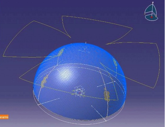
Example: Consider half of a pressure vessel that consists of a spherical cap with a
cylindrical body. If the seed point is on the cylindrical body, which has zero Gaussian
curvature and is developable, limited shearing only occurs over the spherical section.
By contrast, if the seed point is on the spherical section, shear builds up rapidly and the
surface cannot even be covered.
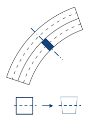
Seed Curve
A seed curve forces the warp, weft, or bias directions of the fabric along a curve.
The curve must pass through the seed point, and extend to the ply boundaries. In the
following example, the bias direction of the fabric has been forced along a curve through
the middle of the spar. This results in a flat pattern with parallel sides, which is a
tape.
The choice of whether the warp, weft, or bias directions are forced along the curve depends
on the relative alignment of the nominal warp and weft directions at the seed point, and the
seed curve at this point.
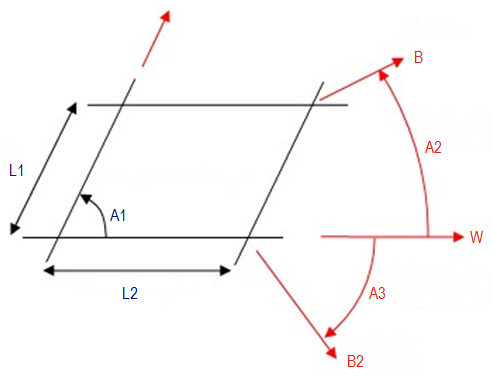
The woven construction of the fabric is defined by physical parameters that reflect the
structure of the material.
In the image below:
- L1: Weft Length
- L2: Warp Length
- A1: Warp/Weft Angle
- B: Bias, B2: Bias2
- A2: Warp/Bias Angle
- A3: Warp/Bias2 Angle
- W: Warp
In Composites Fiber Modeling, the Warp/Weft Angle is defined under Simulation:
Advanced parameters, and information is found under Material
parameters, whereas the Warp and
Weft length ratio is defined under the Mesh
parameters. For the purposes of defining the unit cell, it is the ratio of
warp and weft lengths that is important. So, if warp and weft lengths are the same, the bias
directions are at +/- 45 degrees.
The axis forced along the seed curve is the closest to the seed curve at the seed point.
For example, if the Warp/Weft Angle is 90 degrees and the warp and
weft lengths are identical, and if the seed curve lies 30 degrees from the nominal warp
direction, the bias direction is closest to the seed curve and this is the direction forced
along the seed curve.
This snapping to the nearest direction means that the actual and nominal warp directions at
the seed point can be slightly different - 15 degrees in the case above. This must be
accounted for when using the inspection tool.
The seed point must be located on the seed curve. In practice, a tolerance of 1% of the
square root of the ply area is allowed to permit small separations between seed point and
seed curve resulting from the thickness update capability, for example.
Guide Curve Options
You can select the way the warp angle is calculated with respect to the guide
curve.
- Snap to Axes
- The initial warp direction at the seed point is calculated with respect to the guide
curve. The closest of the material warp, weft, or bias directions are created on the
guide curve.
This results in a robust solution but means that the actual warp
direction is not necessarily the same as the theoretical direction. The image
below shows the bias points of an initial producibility mesh being snapped to the
guide curve, resulting in a warp direction differing from the theoretical direction at
the seed point.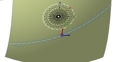
- Constant Angle
- The initial warp direction at the seed point is calculated with respect to the guide
curve, and the warp angle is kept constant at this value along the whole guide curve.
If the theoretical warp/weft or bias directions are within 0.1 degrees of the guide
curve at the seed point, that axis is snapped onto the guide curve to promote
robustness of the solution. The image below shows the initial producibility
mesh at an angle of approximately 30 degrees to the guide curve, with the actual warp
direction matching the theoretical direction at the seed point.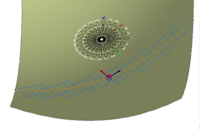
Note:
The strong constraint provided by these two options may prevent a stable simulation on
highly curved surfaces with a guide curve.
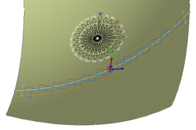
- About Curve
- A producibility mesh of one cell width is draped along the guide curve. As this strip
is narrow, little shearing of the material is introduced.
This option models
unsheared material being forced along the guide curve, followed by subsequent lateral
laydown to the edge of the ply. Note:
This constraint may lead to the need to
insert a split into the material in the same way as for an Order of Drape simulation
with a concave edge.
Order of Drape
The order of drape capability allows you to model the exact sequence used to apply
fabric to surfaces on the shop floor.
The order of drape regions define smaller surfaces that are covered in one sequence, and which provide a stable initial condition for subsequent application
of material.
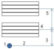
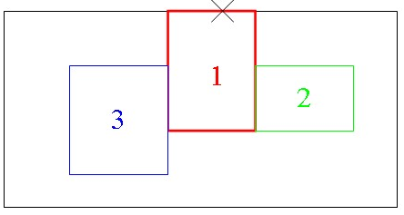
In the example below, three order of drape regions are defined:
- The first order of drape region marked in red (1) must contain the seed point (X),
otherwise it is ignored.
- At the end of the first sequence, the area defined by the second order of drape region
marked in green (2) is covered by fabric using the first order of drape as a starting
point.
- The third order of drape region (3) is similarly covered next.
- Finally, all the remaining area of the ply is covered.
Do not define too many order of drape regions on a single ply. Usually, between one and two
regions are sufficient.
Try to define order of drape regions on relatively flat regions of the surface: The
position of the seed point is not significant, and this lack of sensitivity follows through
the simulation, resulting in a robust final result, that is easily manufacturable.
In general, it is best if the summed boundaries of all the order of drape regions are
straight or convex. If they are concave with respect to a warp or weft fiber, the fiber in
the fabric might be over-constrained as shown below.
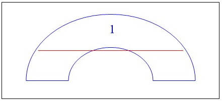
Here, the first order of drape region will drape perfectly well with its shape. But
consider the red fiber as the drape extends beyond the first region. Here, the fiber
suddenly becomes over-constrained as the drape extends across the concave boundary, so that
the fibers become kinematically inadmissible.
To handle this situation, Composites Fiber Modeling unsticks fabric on one branch of the semi-circle (keeping the branch where the red line
is longest) to remove the excessive constraint. This behavior is followed if the
Inadmissible Mode is specified as Delete, that is, the
constraint is deleted as required. Note:
The flat pattern over the order of drape region can
change in subsequent drapes.
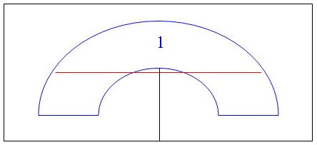
This situation of kinematic inadmissibility can be resolved by placing a dart in the middle
of the semi-circular region using the limit contour capability as shown below. This dart
removes the excessive constraint and allows draping to proceed.
You can force Composites Fiber Modeling to keep the fabric stuck to the order of drape regions during subsequent extensions if
Inadmissible Mode is specified as Cut. In
this case, kinematically inadmissible fibers are avoided by automatically generating a rough
cut in the middle of a bounded length in an over-constrained fiber, such as that shown in
red in the figure above. This cut is created only if the strain required in the fiber to
allow it to conform to the surface exceeds the inadmissible tolerance value set, or the
displacement mismatch at the cut location exceeds half a step length in the appropriate
direction. This approach has the advantage of keeping the flat pattern in an order of drape
region constant during subsequent draping, but forces you to define a dart to specify the
flat pattern shape around the dart accurately. This methodology is suitable for highest
accuracy on components like curved frames where it is impossible to avoid concave order of
drape boundaries.
Seed curve and order of drape can be combined if required, but the seed curve (and seed
point) should lie in the first order of drape region.
For CFM FEFlatten propagation types, the Edge smoothing distance
parameter controls to which degree the material sticks to the surface:
- In this method, a given 3D surface geometry is meshed with triangular finite elements
that are as close in size and shape as possible within the constraints of the geometry
and chosen step length. The element associated with the Seed Point is then defined on a
2D flatten plane and adjacent elements are laid down in a radially expanding way until
the edge of the ply is reached. Double curvature in the surface means that both the new
element and the already-flattened elements are geometrically incompatible and have to
deform when connected.
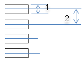
- When a new element is added to the flatten shape, only already-flattened elements
within this distance to the free edge are allowed to deform, while other elements are
fixed. Below, the cross represents the seed point. The solid line represents the free
edge. The Edge smoothing distance is the distance between the
solid and the dotted line.
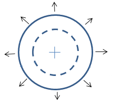
The default
distance value (20mm) represents the size of a finger or a tool used to drape material
over a surface.
Notes:
- As the Edge smoothing distance increases, the material
becomes increasingly free to move while being draped and the solution tends toward the
CFM FEFlatten (Frictionless) solution, which reflects the
limiting case where the material is completely free to move with respect to the
surface.
Unlike direct simulations of material fibers, the FEFlatten solution can
accommodate holes in the underlying ply surface as it can encircle holes.provided
the holes are smaller than Edge smoothing
distance.. Default material properties are isotropic, but
orthotropic materials are supported. For orthotropic properties, if the shear
stiffness is much less than the stiffnesses along the fibers, the material deforms
in a very similar way to the “pin-jointed net” material model used in other fiber
simulations provided the deformation is relatively small.
Smooth Regions
A smooth region is an area where the simulation can ignore awkward bumps/hollows for
an initial global simulation. The subsequent local draping goes from the smooth region
boundary toward the middle of the bumps/hollows.
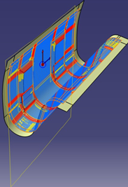
Many composite structures contain "bumps" - a ubiquitous example is that of a sandwich
panel incorporating cores. When laying plies over the bumps, the material necessarily shears
to conform to the highly curved surface covering the bumps. This shearing deformation is
indicated by the red fibers on the J-panel below.
However, it is often required to define plies that lie around the bumps, but do not cover
them. As most fiber simulations cannot accept holes in the surface used for simulation, the
underlying surface that includes the bumps is used for the simulation, so high shear is
still predicted whereas the surface excluding bumps may be rather simple and not need
excessive shear.
Draping result with smooth regions

The smooth region is defined by an area and a curve.
- The area, with or without an order of drape, specifies a developable region.
- The smooth region curve defines a bump inside to be filled with a smooth surface using
point, tangent, or curvature.
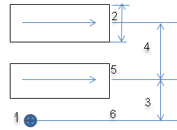
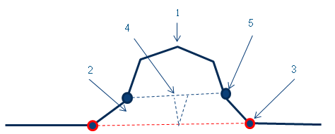
In the image below:
- 1 represents the bump.
- 2 represents the manual trimming area.
- 3 represents the smooth region boundary.
- 4 represents the required dart.
- 5 represents the finished inner boundary.
The example below has an interior contour. Without a smooth region, draping occurs over the
entire surface causing strain to be distributed in places where it is undesirable. With a
smooth region curve:
- The smooth region is filled with a surface and combined with the ply shell.
- This new smooth surface is simulated to create a low strain surface giving good
edges.
- Next, the area inside the smooth region curve is added, and any strain is propagated
into this region. Generally, causing the need for darts.
- The blue arrows show the interior contour. The pink arrow shows the smooth region
curve.
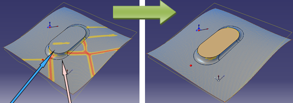
- This is the difference of flat patterns.
Notes:
- The smooth region boundaries should not cross ply boundaries (possibly modified by
darts) nor order of drape region boundaries. If an inner ply boundary lies inside a
smooth region boundary, dart the material at the inner boundary. If you do not define
darts, the simulation proposes rough darts as the models for the darts to define. The
inner darts should extend to the smooth region, but not cross it.
Mesh Parameters
The Mesh parameters define the architecture of the fabric, and
the step lengths used for the fiber simulation.
Regarding the architecture of the fabric, the ratio between warp and weft is constant for a
particular material. Use this material property consistently. This is especially important
when using a seed curve.
The fiber simulation in Composites Fiber Modeling is relatively insensitive to step length. This makes the
simulation accurate for highly curved surfaces, and reduces sensitivity to step length.
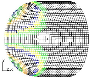
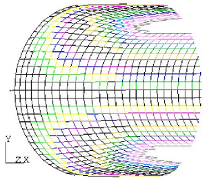
Consider the following channel section. For a wide variety of step lengths (between 1 and
50 mm), the Composites Fiber Modeling result predicted the same flat pattern. By contrast, the
standard fiber simulation gave very different results depending on the chosen step length,
and large step lengths lead to very poor flat pattern results.
As a result of the insensitivity to step length, there is no need to have very small step
lengths and this can, in fact, be counter-productive.
Fine detail on the edge of the ply is picked up irrespective of the step length.
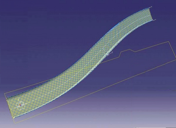
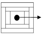
As you can see in the image below, the warp and weft lines (blue) at the spacing requested
by the user have crossed the line defining the ply boundary (orange) at the location marked
with circles (green).
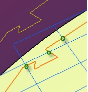
The line showing the flat pattern (yellow) still contains the fine detail of the edge,
which reflects the local strain in the ply.
There is no need to specify a small spacing to pick up details. The
Note:
Fiber visualization does not reflect that the underlying simulation in Composites Fiber Modeling follows the underlying surface exactly. This is a property and does not reflect the
accuracy of the results.
Propagation Type
The propagation type reflects the way in which the fabric covers the surface. As a
consequence, different propagation types lead to different shapes and measures for the
flattened ply.
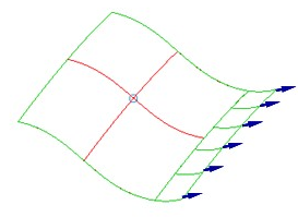
Consider fabric placed on a surface beginning at the seed point with the principal warp and
weft fibers defining seed curves being shown in red below. If the red lines are constrained
to the surface, the placement of the fabric bounded by the green line is then uniquely
defined.
Extending the material further to the ply boundary is done one free edge at a time. When
extending a free edge, the fabric behaves as a trellis and so the exact direction of growth
is not fully defined. Therefore, assumptions must be made of the direction of growth based
on the material behavior and manufacturing method. Composites Fiber Modeling provides several different propagation modes to cover the
most important manufacturing options, that fall into three categories.
- Optimized Energy and Optimized Maxshear
modes use a biaxial material model and a circular extension strategy to model the hand
layup of woven fabrics.
- Second, the Tape Steering and Tape Angle
modes use a strip extension strategy to simulate the application of biaxial or uniaxial
tape respectively in a way that accurately reflects the real-world application of butted
tapes of material onto a surface by manual means. This is also likely to reflect butted
tape laying by automated means, subject to the detailed characteristics of the tape
laying machine are not known by Composites Fiber Modeling.
- Finally, the FEFlatten propagation mode predicts the flattening
of plies using finite element analysis techniques and is applicable to fabrics without a
biaxial or uniaxial microstructure.
Circular Propagation Modes
In the circular extension modes (Optimized Energy and
Optimized Maxshear), free edges in the warp and weft directions are
extended alternately so that the ply extends uniformly in all directions away from the seed
point. This models the operator progressively smoothing the fabric onto the mold away from
the seed point.
- Propagation with circular strategy: Alternate warp and weft extension (the arrow
shows the warp direction):
The two options reflect different shear load deflection-behavior of the ply material. The
best indicator of behavior is a graph of the shear stress/strain response of the material.
Typical stress-strain curves are shown below, with:
- Vertical axis: Load
- Horizontal axis: Deflection
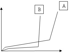
Typically, after a small elastic range, the material begins to shear significantly with
little resistance. This continues up until the warp and weft fibers begin to lock, and
stiffness increases rapidly. The range of behaviors is wide and depends on the weave
architecture, presence of binder, and many other factors.
- In general, Optimized Energy propagation type that seeks to
minimize the shear strain energy on an extending (propagating) edge gives excellent
results for a wide variety of fabrics.
- On the other hand, if locking occurs suddenly in the fabric (as in curve B above),
it is better to limit the maximum shear as much as possible. In this case, the
Optimized Maxshear propagation mode is more suitable.
- Whatever propagation mode, excellent results can be obtained as long as the material
is cut to a net shape, the seed point is accurately located, and the material is
applied with due reference to the ply edge.
A drape using a circular propagation
mode is shown below (the red arrow shows the application). The area of least shear
spreads away from the start point along the principal axes. The amount of shear is
minimized by the algorithm actively working to limit the shear, as a skilled
operator would do.
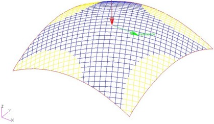
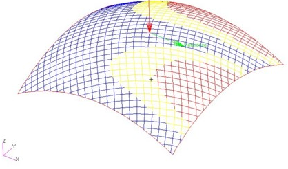
- Geodesic propagation mode extends principal geodesic lines
from the Seed Point to the ply boundary (or the boundary of the
first order-of-drape region, if smaller) in the initial directions of warp and weft
yarns. This uniquely constrains the fabric bounded by the principal fibers. If draping
continues beyond this region, geodesic fibers are extended as required in warp and
weft directions from points closest to the principal fibers until the surface is
covered.
This propagation type gives good results on surfaces of low curvature, but
can lead to excessive shear for regions of high curvature.
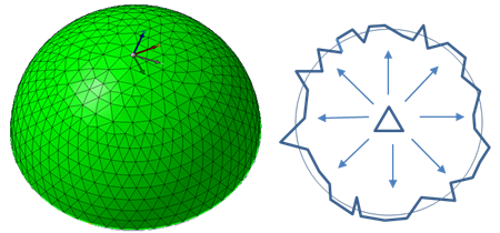
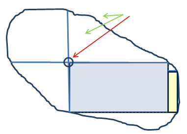
In the image below
- The green arrows point to the seed points.
- The red arrow points to principal fiber along geodesic path.
- The blue rectangle represents the constrained region, the yellow one the
extension nearest principal fiber.
- Energy (Frictionless): In general, simulations of hand layup
assume that the fabric sticks to the surface completely as soon as it is smoothed onto
the surface. This is an appropriate assumption for most hand layup materials and
processes, but has the effect of locking in excessive material deformation.
Energy (Frictionless) propagation mode models the case of no
friction between fabric and mold. It allows the fabric to move to minimize the
overall shear strain energy in the material. This yields a unique solution for a
particular Seed Point (which should instead be considered as
a Reference Point) and initial warp direction and indicates idealized fiber paths
that minimize overall ply deformation. Also to be used to estimate deformation
during matched die forming. Note:
Energy (Frictionless) is intended to model forming between
two frictionless forms, and uses an iterative solution to minimize the shear
strain energy throughout the ply. This means that the material may shear at the
indicated point, which is a Reference Point and not a Seed Point. The solution
should not be highly dependent on the location of the Reference Point, but
computationally the best location for this point is near the center of the ply -
so the Geometrical Center option is suggested as a starting
point.
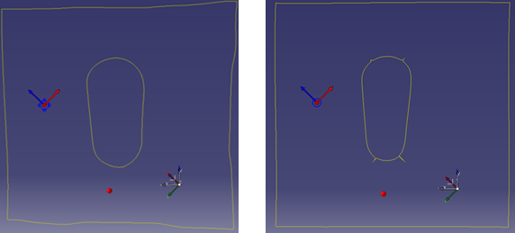
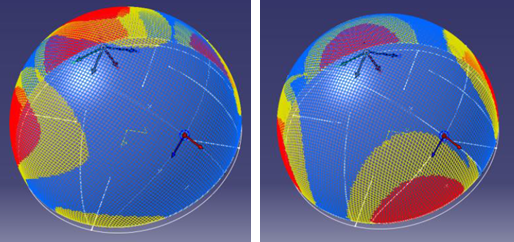
A comparison between results from the Optimized Energy (on
the left) and Energy (Frictionless) (on the right)
propagation modes for a non-symmetrical seed/reference point is shown below.
Energy (Frictionless) acts to reduce shear despite the
reference point not being in the middle of the ply.
Energy (Frictionless) runs an initial Optimized
Energy solution and then iterates the results to minimize shear strain
energy. The solution is therefore an order of magnitude slower and can be less
stable than standard results.
Strip Propagation Modes
Another propagation mode is the strip propagation.
Suitable to simulate the layup for ATL (Automated Tape Laying) and AFP (Automated Fiber
Placement) machines.
In general, the first tow is laid down and subsequent tows are laid parallel until the
end of the ply. The principal path passing through the Seed Point is determined by one of
three methods:
- Priority Angle, where the principal path follows the theoretical projected path on the
surface. This choice minimizes Deviation.
- Priority Steering, where the principal path follows a geodesic path on the surface.
This minimizes Deformation.
- Guide Curve, which is a manually defined curve to allow for a custom solution.
From the initial path, subsequent paths are generated parallel to it in the plane of the
surface.
Tape Steering:
- The first tape is extended from the seed point in the warp direction all the way to
the ply boundary in both the positive and negative warp directions.
- Only once this first tape is laid are additional tapes abutted against the free weft
edges of the preceding tapes.
- For each new tape, the material strain is zero at the point of first application,
which is defined as the point in the most negative warp direction. This reflects that
the material is unsheared at the point of first application on a surface. The rate of
increase of shear along the tape depends on the width of the tape and the Gaussian
curvature of the surface.
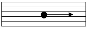
- Propagation with strip strategy: Initial warp extension, then lateral weft (the
arrows show the warp direction)
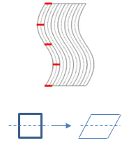
- For standard biaxial material model, it is assumed that warp and weft fibers pivot
about their cross-over points so that an initially square piece of material becomes a
rhombus after shearing in a scissor mode as shown below.
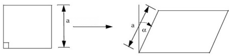
Importantly,
the lengths of the sides remain constant as they are sheared.
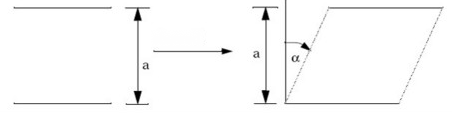
- Alternatively, for uniaxial materials, parallel fibers are assumed to remain
parallel and equidistant, with shearing resulting from the relative sliding of
fibers.
In practice, the results of the two material models converge on the same solution for
small shears. At higher shears, the warp fibers of a biaxial material close up, which
tends to reduce the amount of shear in a ply covering a surface of positive Gaussian
curvature.
A drape using the Tape Steering propagation model is shown
below.
Notes:
- The shear is zero along the principal warp direction as in this case, this follows
a geodesic line on the surface.
- The shear is zero by definition at the minimum warp end of each tape.
- The degree of shear is higher than for the circular algorithm above.
In the strip extension mode Tape Angle, the principal fiber
follows the theoretical direction (projected Rosette X-Axis, rotated through the ply angle
in the plane of the surface) to the edge of the ply. This means that the deviation along
the principal fiber is null.
Tape Steering and Tape Angle both propose a
deformation model that can be set to either .
FEFlatten Propagation Mode
The circular and tape propagation modes mentioned previously are based on a
geometrical fiber simulation and give excellent results for Uniaxial and Biaxial materials
where the material deforms in a highly directional way with almost no deformation along the
fibers and concentrated deformation between fibers. However, some materials used for
Composites parts behave in a more isotropic manner with the material deforming in a
direction imposed by the applied force and tractions within the ply rather than forced in a
particular direction due to the underlying fiber architecture.
These include the following sheet materials commonly used in the manufacture of laminated structures:
- Quadraxial Non-Crimp Fabrics (NCF)
- Chopped Strand Mat (CSM)
- Knitted Fabrics
- Foam Cores
- Vinyl and Leather
To calculate the flat and draped patterns of these materials, a purely geometrical
approach cannot identify the important load paths in the fabric as it is forced over a
doubly curved surface and instead a finite-element based flattening (FEFlatten) solution
is required.
The finite element flattening approach:
- Effectively calculates the initial flat shape of the ply assuming that the material
is formed between two frictionless dies. This allows the calculation of a smoothed
minimum energy solution over the whole ply. The solution is a sophisticated extension
of the approach of McCartney et al (1999, 2005) coupled with the use of nonlinear
finite element analysis techniques.
- The solution time can be expected to be of the order of minutes.
- This technique can be thought of as lying between a purely geometrical simulation,
taking seconds, and a full-contact multi-ply finite element calculation, taking
days.
- A particular advantage of the FEFlatten solution is that
interior holes can be free boundaries, so that surfaces containing holes (or
bumps/hollows surrounded by interior contours) can be solved without problems.
- A comparison between geometrical fiber simulation and finite element flattening
approaches is given in the table below:
|
Geometrical Fiber Simulation
|
Finite Element Flattening
|
|
Initial value problem, local energy minimization
|
Boundary value problem, global energy minimization
|
|
Exact flatten around details
|
Flatten smeared by finite element definition
|
|
Solution in seconds
|
Solution in minutes
|
|
Holes cannot be free boundaries
|
Holes can be free boundaries
|
|
Uniaxial, Biaxial materials
|
Isotropic, general materials
|
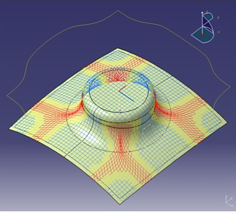
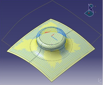
A comparison of simulation results obtained through the standard Composites Fiber Modeling geometrical solvers, and the Composites Fiber Modeling flattening solver, for a mesa-like protuberance on a
gently curved surface is given below. This clearly shows that by allowing strain along the
fibers, the FEFlatten propagation mode reflects the reduction of
peak strains in the material.
|
Geometrical Fiber Simulation
|
Finite Element Flattening
|
|
Pin Jointed Net
|
Finite Elements
|
|
Pure Shear Strain
|
Shear + Normal Strain
|
|
Concentrated Deformation
|
Distributed Deformation
|
|
|

|

|
Display Modes
The 3D draped pattern for Composites Fiber Modeling is displayed in the same way as the standard fiber
simulation.
The result can be used for inspection and 2D-3D transfer, and can be stored as curves in
the model.
Note:
The graphics visualization does not reflect the underlying simulation completely in the
following respects:
- Composites Fiber Modeling follows the surface exactly, whereas the
visualization only joins points on the surface.
- Composites Fiber Modeling continues the simulation to the edge of the ply,
whereas the visualization does not allow the display of partial fibers and so the
"Lonely Points" are removed.
When using the enhanced producibility panel, users can access specialized display modes relevant to the
fiber simulation. These give additional insight into the deformation of the ply over and
above the degree of pure shear visualized in the standard Shearing
Angle display mode. Composites Fiber Modeling currently supports display of the Steering
Radius (not FEFlatten), and Axial Strain (only CFM
FEFlatten).
Steering Radius (Not FEFlatten)
The steering radius is the radius of curvature of the fibers in the plane of the surface.
This information is particularly useful for investigating the viability of tape laying,
where the forming limits of tape are usually characterized by the minimum manufacturable
radius of curvature.
The steering radius is also an additional measure of the degree of deformation in fabrics
and can complement the standard shearing angle display.
Axial Strain (Only FEFlatten)
The FEFlatten solver admits the possibility of axial strain along the nominal warp and
weft fibers. It is only valid for the FEFlatten solver as the value would be zero for
other solvers.
Maximum Slope
Thickness Update provides a powerful capability to offset the
simulation mesh from the ply definition surface. The result is a very accurate flat pattern of
plies offset from the mold surface (far better than offsetting by a constant thickness).
However, for complex layups, there are situations where the resultant updated surface becomes
uneven.
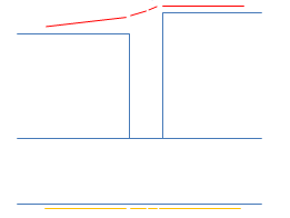
As an example, consider the case of a two plies that are separated by a small gap (This may
be intended by the designer to promote resin flow).
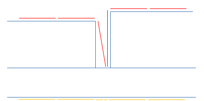
Here, the surface
simulation mesh (in yellow at the bottom) is necessarily defined to respect ply boundaries
on the surface, but when updated, results in a surface (in red on top).
Since Composites Fiber Modeling produces very accurate flat patterns as it follows the
surface absolutely, it is disproportionately affected by surface quality. In fact, the
surface roughness described above is seamlessly handled by Composites Fiber Modeling, but the effect of generalized crossing of hundreds of
ply boundaries can be unpredictable. To solve this problem while taking advantage of the
power of Thickness Update, smooth the simulation surface by choosing
a maximum slope of the offset facets measured from their baseline position as shown below.
This effectively
removes simulation surface artifacts and results in stable simulations with better
results.
Display Flat Pattern
Composites Fiber Modeling computes the flat pattern instantaneously as an intrinsic
feature of its simulation.
This ensures:
- Accuracy, as it is an intrinsic part of the simulation process,
- Speed, as no separate process is involved.
- Clarity, as it is possible to visualize the 2D flat pattern at the same time as the 3D
draped pattern.
To display the flat pattern at the same time as the draped pattern, select the
Display Flat Pattern check box. The flat pattern is displayed in a
plane parallel to the surface at the seed point, and with the correct orientation.
The feedback allowed by this feature gives the user immediate confidence in the quality of
the fiber simulation.
|