Analyzing Using Porcupine Curvature | |||||
|
| ||||
-
From the Analysis section of the action bar, click Porcupine Curvature Analysis
 .
.
- View the quick analysis on a curve:
- In the Type area, select Radius.
- Select the Quick tab.
- In the Radius box, type the value or use the arrows to change the value.
-
Select a curve.
The parts of the curve having radius value less than the specified tolerance value are displayed in red color.
 Note: You can double-click the color bar available before the Radius box to configure the color.
 - In the Type area, select Curvature.The parts of the curve having curvature more than the specified tolerance value are displayed in red color.
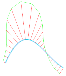
- View the comb analysis on a surface and then on a curve:
- Select the Full tab.
-
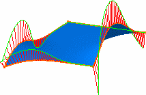
Select a surface.
- If you select the surface, the porcupine comb shows the curvature on each boundary of the surface.
- If you select a specific boundary, the comb is displayed only on this boundary. Ensure the Geometrical Element Filter selection mode is active from App Options
> User Selection Filter (this mode lets you select sub-elements).
- If you select the surface, the porcupine comb shows the curvature on each boundary of the surface.
-
Select a curve.
The porcupine comb shows the curvature of the curve.
- In the Type area, select Radius.The porcupine comb now shows the radius of the curve.
- Adjust the characteristics of the porcupine comb:
- In the Type area, select Curvature.
- In the Density area, adjust the number of spikes in the comb by using either of the following methods:
- Type the value or use the arrows to change the value.
- Click X2 and /2.
In this example the density of the spikes has been increased.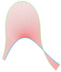
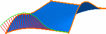
- In the Amplitude area, adjust the length of the spikes in the comb using either of the following methods:
- Type the value or use the arrows to change the value.
- Click X2 and /2.
In this example, the amplitude of the spikes has been decreased.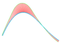
Notes:- Adjusting the density of the spikes is particularly useful when the geometry is too dense to be read but the resulting curve may not be smooth enough for your analysis needs.
- If the Automatic check box is selected, the length of the spikes is optimized so that the spikes are always visible, even when zooming in or out.
- If the Variable Auto check box is selected, an individual zoom factor is applied to each selected curve.
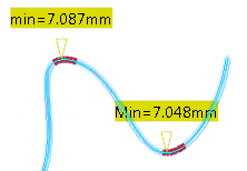
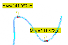
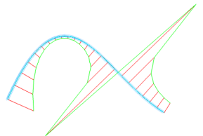
- Click Min value
 and/or Max value
  to display the minimum or maximum points or both.
Note:- Inflection points appear only if Project on Plane, Min value, or Max value options are selected.
- You can click Inverse Value to display the inverse values for Radius when Curvature is selected or for Curvature when Radius is selected.
Note: Contextual commands are available when you right-click Min value or Max value; they apply to all the curves involved in the analysis. - View a curvature diagram:
- In the Diagram area, select Display diagram window
 .The 2D Diagram dialog box appears.
The curvature amplitude and parameter of the analyzed curve are represented in this diagram.
Note:- In the curvature graph, the X axis abscissa is curvilinear when Curvilinear is enabled in the Porcupine Curvature dialog box, otherwise the X axis abscissa is parametric. When X axis abscissa is parametric, its range is not necessarily between 0 and 1.
- The X axis abscissa values are independent of the selected type of curvature analysis, Radius or Curvature.
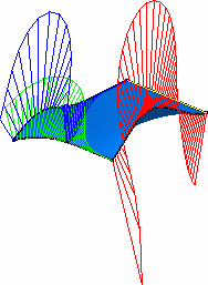
When analyzing a surface or several curves, you can use different options to view the analyses.
For example, when analyzing a surface, by default you obtain this diagram, where the color of the curves in the 2D Diagram dialog box match the ones on the geometry.
- Move the cursor over the porcupine comb in the work area.The local amplitude is displayed and the current location is displayed in the 2D Diagram dialog box.
- Right-click a curve in the 2D Diagram and choose one of the following
options:
- Remove: removes the curve.
- Drop marker: adds Points.xxx in the specification tree.
- Change color: displays the Color selector dialog box that enables
you to change the color of the curve.
Important: Users colors are lost when you close the curvature graph dialog box.
- When you have finished with the 2D Diagram, click the x in the top right corner to close.
- In the Diagram area, select Display diagram window
Notes:
- The Reverse analysis is opposite to that which was initially displayed. This is useful when, from the current viewpoint, you do not know which way the curve is orientated.
- The Project on Plane option applies a curvature signature due to the curvature analysis projection.
- The Plane curves option projects the porcupine analysis on a mean plane, if one exists within the given tolerance.
- In case of clipping, you may want to temporarily modify the Depth Effects' Far and Near Limits. For more information, see 3DEXPERIENCE Native Apps: Native Apps Advanced: Additional Viewing Commands: Setting Depth Effects.