Eigenstrain-Based Simulation of Additive Manufacturing Processes
Abaqus/Standard
offers a general framework for eigenstrain-based simulations of additive
manufacturing processes.
This section provides an overview of special techniques that are
available for, but not limited to, eigenstrain-based simulations of additive
manufacturing processes. These techniques can be applied to other processes,
such as welding.
An eigenstrain analysis of additive manufacturing processes:
is a computationally efficient method for the prediction of part-level
distortion and residual stresses introduced during the additive manufacturing
process;
consists of a single stress analysis with a predefined set of
eigenstrains that are applied to each element upon activation and that
represent the inelastic deformation induced by the processes;
simplifies the definition of the problem by eliminating the need to
specify detailed processing conditions;
is generally a more approximate solution with a shorter modeling and
simulation time than a thermal-stress analysis; and
can be followed by analyses of support removal, and/or mechanical
performance tests, etc.
Residual stresses in mechanical parts are stresses that exist in the absence
of externally applied loads. Almost all manufacturing processes, including
additive manufacturing, introduce residual stresses into mechanical parts.
Residual stresses are sometimes introduced intentionally to improve the
in-service response, such as in prestressed concrete slabs used in bridge
construction. However, manufacturers often try to minimize residual stresses
because they can cause fracture during the manufacturing process, lead to
unwanted distortions, and significantly impact fatigue behavior. Three primary
classes of manufacturing effects lead to residual stresses:
Mechanical (for example, inelastic deformation);
Thermal (for example, nonuniform thermal expansion or incompatible
thermal strains generated during melting and solidification in the process
zone); and
Changes in material microstructure (for example, phase transformations).
Eigenstrain (also referred to as inherent strain, assumed strain, or
"stress-free" strain) is an engineering concept used to account for all sources
of inelastic deformation that lead to residual stresses and distortions in
manufactured components. Thermal strains are a subset of eigenstrains.
In a linear elastic deformation, the stress induced by an eigenstrain can
be represented as
where
is the Cauchy stress;
is the elastic matrix;
is the total strain;
is the eigenstrain; and
is the elastic strain.
Using constitutive equations (such as the one shown above) eigenstrains can
be used to compute residual stresses coming from mechanical, thermal, and
microstructural sources.
An eigenstrain in three dimensions is represented as a standard strain
tensor with six components:
The components of the eigenstrain tensor are functions of many factors,
including material properties, manufacturing processes, and thermal history.
Various methods can be used to determine appropriate eigenstrains for a given
process:
Destructive and nondestructive tests of manufactured parts.
Numerical simulation.
Analytical formulas for simple scenarios.
Once an appropriate eigenstrain field has been determined, it can be
applied in an eigenstrain analysis to predict the distortions and residual
stresses in an additive manufactured part.
Eigenstrain-Based Simulation of Additive Manufacturing Processes
An eigenstrain analysis of an additive manufacturing process consists of a
single static stress analysis of a printing part with a predefined field of
eigenstrains that are applied to each element upon activation representing the
inelastic deformation induced by the process. These inelastic deformations
become the main source of residual stresses and overall part distortion;
therefore, the objective of an eigenstrain analysis is to predict distortions
and residual stresses in the part. Eigenstrains applied to a newly deposited
layer can induce residual stresses and distortion on layers underneath.
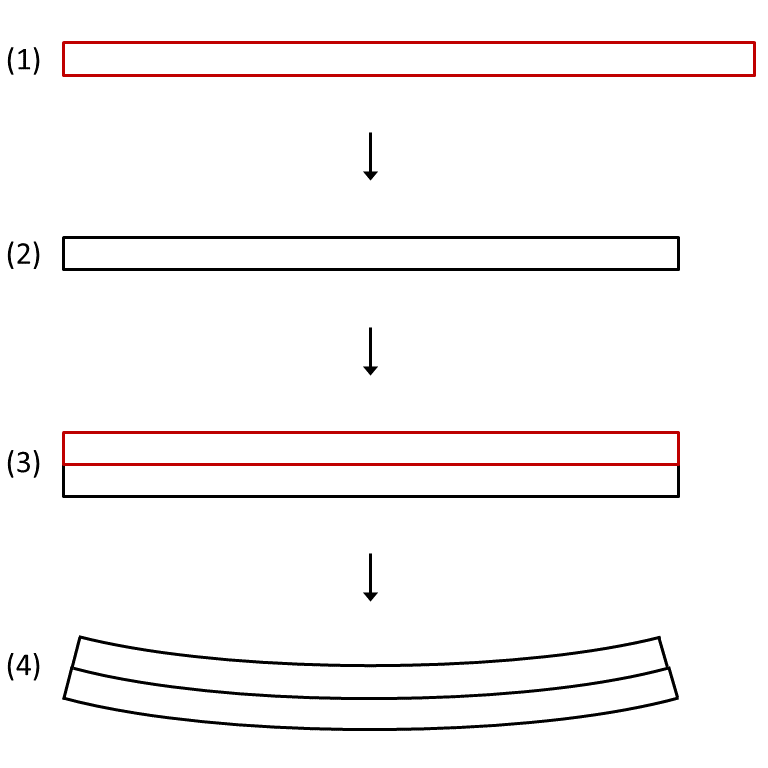
Figure 1
shows a simple example of an additive manufacturing process of a two-layer
build with the following conditions:
The first layer is added.
The first layer is unconstrained—it contracts when negative eigenstrains
are applied.
The second layer is added on top of the first layer and bonded to the
first layer.
The contraction of the second layer is constrained by the bonding of the
first layer, causing the part to distort and inducing residual stresses.
The eigenstrain analysis can also include support structures (if required
for the build) and a substrate where the part and support are built to consider
their influences on part distortions and residual stresses. In general, an
eigenstrain analysis provides a more approximate solution than a thermal-stress
analysis. However, because only a static procedure is required, an eigenstrain
analysis often has a shorter run time.
Distortion due to eigenstrains in a two-layer additive manufacturing
process.
Progressive Element Activation and Eigenstrains Application
Material deposition in the additive manufacturing processes is modeled in
Abaqus/Standard
by progressive element activation (see
Progressive Element Activation).
Elements are activated in either a full or partially full state. In each
increment during an analysis, you can use user subroutine
UEPACTIVATIONVOL to control the element activation and the volume fraction
of material added to each element and to define the eigenstrain tensor
associated with the new material (see
Applying Eigenstrains).
Abaqus
automatically applies the eigenstrain to the element, introducing residual
stress in the element.
By using user subroutine UEPACTIVATIONVOL, you have complete
control over the element activation sequence and the eigenstrain values to apply. You can
access toolpath-mesh intersection utilities that are specially designed to define and apply
eigenstrains for common additive manufacturing processes. Two types of eigenstrain analyses support this
functionality: trajectory-based and pattern-based.
Abaqus/Standard also provides streamlined solutions for common trajectory-based and pattern-based
eigenstrain analyses that do not require you to write user subroutines.
Trajectory-Based Eigenstrain Analysis
A trajectory-based eigenstrain analysis activates elements and applies
eigenstrains based upon a specified trajectory of new material being fused or
bonded to the underlying layer. For example, the trajectory of a powder bed
fusion process is the same as the heat source scan path, and the trajectory for
directed energy deposition and material extrusion processes is the nozzle path.
The trajectory is defined using an event series (in the form of time, spatial
coordinates, and user-defined data of events; see
Event series for more details) and processed
directly by the toolpath-mesh intersection module. In user subroutine
UEPACTIVATIONVOL, you can call the relevant toolpath-mesh intersection
utilities to obtain information about the change of volume fraction of material
and the eigenstrain values to assign to each element in each increment.
Optionally, you can update the material orientation to align it with the
trajectory. The analysis is similar to the stress analysis in thermomechanical
simulations, except that it is driven by eigenstrain loadings instead of
temperature results for the thermal analysis.
Pattern-Based Eigenstrain Analysis
A pattern-based eigenstrain analysis activates elements layer by layer and
applies eigenstrain based on a specified in-plane eigenstrain pattern for each
layer. An eigenstrain pattern is a domain that is partitioned by a "quilt" of
one or more patches. Each patch is an area that contains a specific value of
eigenstrains or a rotation angle of eigenstrains as a result of a specific
trajectory in that area. For example, the eigenstrain patterns for powder bed
fusion processes are related to the in-plane scan pattern of the heat source,
and the eigenstrain patterns for directed energy deposition processes and
material extrusion processes are related to the in-plane moving pattern of the
nozzle. A pattern-based eigenstrain analysis does not require you to define a
trajectory. The analysis considers layer-by-layer building sequences and
ignores the detailed sequences of material deposition or scanning within
layers. You define parameters and properties of eigenstrain patterns using
table collections (see
Table Collections, Parameter Tables, and Property Tables)
and access them using user subroutine
UEPACTIVATIONVOL. In the user subroutine you can activate elements in a
layer-by-layer fashion, call the toolpath-mesh intersection utilities to
identify which eigenstrain patch an element in the last activated layer belongs
to, and apply the eigenstrains to the element. You can also update the material
orientation, such as aligning it with the rotation angle of the eigenstrain of
the patch.
Partial Element Activation in Eigenstrain-Based Simulation
Eigenstrain-based simulations in
Abaqus/Standard
are supported with full and partial element activation. In the case of partial
element activation the volume fraction of material added can be arbitrary;
however, in practice the value should be larger than a small threshold value to
avoid numerical singularity problems. Full activation is a special case of
partial activation when the volume fraction of material added is restricted to
1.0.
For partial activation, when new material is added in an increment, both
the old and new material contribute to the stress response of the material. In
general, the two materials might be in different states; therefore, the
homogenized values of state variables are used to compute stresses.
Abaqus homogenizes the variables using the rule of mixtures in which
the variables are computed using the volume weighed average values. For
example, for the linear elastic material model the response is computed from:
where
is the volume fraction of the material in the element; and
is the homogenized elastic strain.
In general, the new material is added with the eigenstrain prescribed. In
this case the homogenized elastic strain is computed from the relation
where
is the volume fraction of the material in the element in the previous
increment;
is the volume fraction of the material added to the element
();
is the total strain increment;
is the eigenstrain in the material added; and
is the elastic strain at the end of the previous increment.
The configuration at which the new material is added is stress free only if
no eigenstrain is prescribed. If the eigenstrain is specified, it causes a
sudden increase of stress that does not decrease when the time increment is
cut. This behavior can cause convergence difficulties, particularly when
geometric nonlinearities are taken into account and nonlinear material models,
such as the elastic-plastic model, are used. In such cases
Abaqus
provides the option of ramping up the eigenstrain linearly in the specified
time interval (see
Progressive Element Activation).
However, you must use caution when choosing the ramping time value; it should
be small relative to the analysis so that the results are not strongly
affected.
Displacement Output
When using progressive element activation in
Abaqus/Standard,
you can control the behavior of inactive elements to follow or not follow the
deformation of active elements in the model (see
Controlling the Behavior of Inactive Elements).
The two behaviors are expected to produce similar results in the limit of small
deformation, with the exception of displacements and rotations (U, UT, and UR).
An inactive element that follows the deformation, also referred to as a
"quiet" element, is always present in the model and participates in the
solution, but it produces a negligible contribution to the overall response. In
this case a node attached to inactive elements can experience nonzero
displacements before any of its attached elements are activated. The nodal
output variables U, UT, and UR represent displacements and rotations measured from the
beginning of an analysis, containing contributions of displacements during both
inactive and active periods of a node.
Abaqus/Standard
also provides nodal output variables UACT, UTACT, and URACT corresponding to the displacements and rotations measured from
the time when an element attached to the node is first activated.
An inactive element not following the deformation does not contribute to the
stiffness of the model and does not participate in the solution. Any nodes
attached to inactive elements remain in their initial position. In this case
the nodal output variables UACT, UTACT, and URACT are the same as the output variables U, UT, and UR, respectively.
Regardless of the behavior chosen for inactive elements, the configuration
of an element upon activation is usually different from the original
configuration because nodes shared by active and inactive elements undergo
displacements (see
Initial Configuration).
When an element becomes active, the configuration at the time of activation is
the reference for subsequent element calculations. Therefore, the output
variable E represents strains measured from the time an element is
activated.
Time Incrementation
The time increment used in eigenstrain analyses can influence the final
results. Assume that two eigenstrain analyses are performed to activate a row
of elements using different time increments: a small time increment activating
one element per increment and a large time increment activating two elements
per increment. The initial configuration of every second element is different
between the two analyses, leading to different results of residual stresses and
distortions. You can choose an appropriate time increment for a
trajectory-based eigenstrain analysis by performing a time stepping convergence
study. For a pattern-based eigenstrain analysis, it is recommended that you use
a time increment less than the time taken to process one element layer.
Resolving Convergence Difficulties
In eigenstrain analyses convergence difficulties can occur when elements are
activated and the eigenstrain is applied.
Elements may distort excessively before they are activated and cause
convergence difficulties. In such situations you should specify that inactive
elements follow the deformation to prevent excessive element distortion (see
Controlling the Behavior of Inactive Elements).
The analysis can have convergence issues if large eigenstrains are
applied instantaneously upon element activation. This issue cannot be resolved
by reducing the time increment. To overcome this issue,
Abaqus
provides an option to ramp the eigenstrains over a period of time instead of
applying them instantaneously upon activation (see
Applying Eigenstrains).
Ramping eigenstrains can influence the accuracy of the analysis results. For
example, if the eigenstrains of elements in a layer are not fully ramped when
the next layer of elements is activated, the strain-free configuration of the
newly activated elements is different from the case when the eigenstrains are
fully ramped. You should use a ramping time constant smaller than the time
increment required for processing one layer.
If the material definition includes plasticity, the analysis may iterate
excessively due to the extrapolation scheme used to speed up the solution. You
can prevent this issue by turning off extrapolation (see
Incrementation in Abaqus/Standard).
Input File Template
The following template shows the input for an eigenstrain
analysis: