The toolpath-mesh intersection module computes the geometric
intersections between various toolpaths used in additive manufacturing
processes and a finite element mesh of the part to be manufactured.
A toolpath represents the motion of a given component of a machine tool such
as a laser source, a recoater roller, or a wire-feed nozzle. A toolpath is
defined by a geometric shape attached to a reference point that moves along a
path. The path is defined by connecting a collection of points in space and
time. An event series defines the collection of points. The first field defined
in the event series describes a state of the tool, such as the laser power, the
"on/off" state for a recoater roller, or a wire-feed nozzle. This field is
assumed to be constant between two consecutive points. A zero-valued field
indicates the "off" state of the tool.
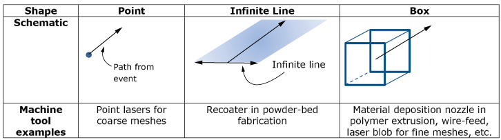
Three shapes are considered for toolpath-mesh intersection: a point, an
infinite line, and a box (see
Figure 1).
These shapes provide different levels of abstraction to characterize the shape
of the tool depending on the particular application. In addition to these three
shapes, a scan pattern that describes the idealized motion of a tool instead of
the actual path of the motion can be used. The topics below list some of the
quantities computed by the toolpath-mesh intersection module for each shape and
a scan pattern. For a complete list of the quantities computed by the module,
see the tables in
Data Retrieval Utility Routines.
Point, infinite line, and box toolpaths.
Point Toolpath-Mesh Intersection
The point representation of the tool shape is useful for situations where
the action zone of the tool is very small compared to the mesh size and can be
idealized as a point; for example, when the laser beam radius is very small
compared to the element size.
Figure 2
depicts intersections of a point toolpath with a finite element,
.
The toolpath is defined by the path connecting points
at times .
It is assumed that the tool travels at a constant velocity over a segment
connecting two successive points in the path. The first field defined in the
event series represents a state of the tool, such as the laser power. The field
defined for a point
remains constant over the segment connecting
and .
All path segments where the tool is in the "on" state are required to be
perpendicular to the global -direction.
For a given element, the toolpath-mesh intersection module computes the number
of intersections of the toolpath, the coordinates of the start and end points
(s
and e,
respectively, expressed in the element reference coordinate system), and the
start and end times (ts and
te, respectively) for each intersection.
Point toolpath-mesh intersection.
Infinite Line Toolpath-Mesh Intersection
The infinite line representation of the tool shape is useful to describe the
process of layer-by-layer material deposition, such as the action of the
recoater roller in powder bed fabrication.
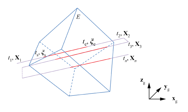
Figure 3
depicts intersections of an infinite line toolpath with a finite element,
.
The toolpath is defined by an infinite line attached to a reference point that
is moving along the path connecting points
such that the reference point is at
at time .
It is assumed that the tool travels at a constant velocity over a segment
connecting two successive points in the path, and the infinite line remains
perpendicular to the segment. The first field defined in the event series
represents a state of the tool, such as the "on/off" state of a recoater
roller. The field defined for a point
remains constant over the segment connecting
and .
All path segments when the tool is in the "on" state must be perpendicular to
the global zg-direction. For a given element,
the toolpath-mesh intersection module computes the number of intersections,
,
of the toolpath and the volume fraction, ,
for each intersection. The volume fraction is equal to the ratio of the partial
volume of the element below the z-plane defined by the
motion of the infinite line following the path to the total volume of the
element. The module also computes the area, A; the
coordinate
with respect to the element reference coordinate system of the center of
intersection of the z-plane and the element; as well as
the area fractions, ,
below the z-plane for all sides (i =
1 to the number of side facets of the element) for each intersection.
Infinite line toolpath-mesh intersection.
Box Toolpath-Mesh Intersection
The box shape functionality is intended for situations where the action of the tool is best
described as a spatially varying distribution. Examples include modeling a Goldak's double
ellipsoid heat source and polymer extrusion material deposition when using fine meshes.
Intersections of a box toolpath and a mesh can be computed using two
different algorithms or approaches; namely, the subsegment approach and the
subelement approach. For both the subsegment and the subelement approaches, the
box length in the local xl-direction can be set
to zero to obtain a rectangular-shaped toolpath.
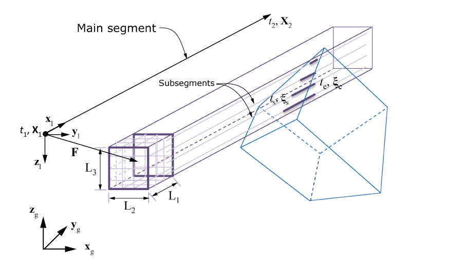
Using the Subsegment Approach
Figure 4
depicts intersections of a box toolpath with a finite element,
,
using the subsegment approach. The toolpath is defined by a box attached to a
reference point that is moving along the path connecting points
such that the reference point is at
at time .
A segment-specific local coordinate system is defined by the vectors
,
,
and .
Vector
is along the segment connecting two successive points, and
is a user-defined vector. The origin of this local system is at the start point
of the segment. The box is oriented along the local coordinate system
directions, and the center is at a constant user-defined offset,
, from the
reference point on the segment. The box lengths ,
,
and
along the local directions are user defined. The box is divided into a
user-defined number of smaller boxes. It is assumed that a subsegment starts at
the center of each smaller box and is parallel to the main segment. A
user-defined weight is associated with each subsegment. The weight is
multiplied with the field associated with the main segment to obtain a field
associated with the subsegment. The sum of the weights of all of the
subsegments is usually equal to one. For a given element, the toolpath-mesh
intersection module computes the number of intersections of subsegments with
the element, the coordinates of the start and end points
(s
and e,
respectively, expressed in the element reference coordinate system), and the
start and end times (ts and
te, respectively) for each intersection.
Box toolpath-mesh intersection using the subsegment approach.
Using the Subelement Approach
In the subelement approach, the box is not divided into smaller boxes.
Instead, the element is subdivided into subelements of the same topology (see
Figure 5).
The number of subelement divisions of an element is set automatically by the
module based on the element size and the minimum dimension of the box. The
toolpath-mesh intersection module computes the number of subelements that have
their centers inside the path of the box, the coordinates of the centers of the
subelements, the volume of the subelements, and the start and end times of the
box passing through the centers of the subelements.
Box toolpath-mesh intersection using the subelement approach.
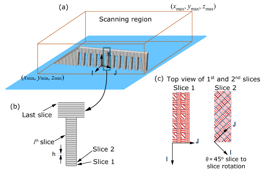
Scan Pattern–Mesh Intersection
Some additive manufacturing processes are characterized by a tool
trajectory that follows a repetitive pattern in space; for example, powder bed
fusion with the laser beam following a predefined island scanning strategy. In
such cases, instead of describing individual trajectories of a toolpath, it is
more effective to define a scan pattern that represents the idealized motion of
a tool inside a part. The part being printed is divided into equally spaced
(uniform thickness, )
slices or cutting planes that are perpendicular to the build axis,
(see
Figure 6(a)
and
Figure 6(b)).
The build axis system
I–J–K is a
user-defined coordinate system that indicates the printing direction,
K. A scan pattern is a representation of the movements of
a tool that is moving or scanning regions of a cutting plane or slice.
A scan pattern with four pattern patches.
The scan pattern consists of a rectangular unit cell (see
Figure 7).
The rectangular unit cell is repeated to cover the cutting plane. The
rectangular unit cell consists of a number of smaller rectangular patches. Each
patch can define a local angle, ,
between the direction of the scanning motion of the tool and the
I-axis. You can assign an eigenstrain tensor to each of
the pattern patches representing the inelastic deformation induced by the
process. You can define a scan pattern by defining extents of individual
patches (xmin,
ymin) and
(xmax, ymax).
All patches together must form a rectangular unit cell that must be situated
entirely in the first quadrant of the
I–J plane, and one corner of the cell
must be at (0, 0).
A scan pattern with four patches with local orientations rotated by
90°, 0°, 135°, and 45° with respect to the I-axis of the
build axis system.
A scan pattern is active inside a scanning region. A scanning region is a
build axis–oriented bounding box defined by its extent
(xmin, ymin,
zmin) and
(xmax, ymax,
zmax) (see
Figure 6(a)).
The height of a scanning region
(zmax–zmin)
must be an integral multiple of the thickness, h, of a
slice. Multiple nonoverlapping scanning regions can be defined to cover the
entire part. A different scan pattern can be active inside each scanning
region. All scanning regions share the same build axis system. A layer-to-layer
or slice-to-slice rotation angle, ,
can be defined. The scan pattern is rotated by
on the
slice for layer
(see
Figure 6(c)).
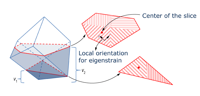
For a given element, the toolpath-mesh intersection module computes the
number of slices, m, inside the element in a given
increment (see
Figure 8).
It finds which pattern patch contains the center of each slice in that element
and the local orientation of that patch considering the layer-to-layer
rotation, ,
and the local rotation, ,
of the scanning direction in that patch. The module also computes the partial
volumes, ,
of the element below each slice.
Scan pattern overlaid on an element.
Supported Elements
Linear and quadratic 4-, 5-, 6-, 8-, 10-, 15-, and 20-node solid elements
and 3-, 4-, 6-, and 8-node shell elements with constant shell thickness are
supported. For shell elements, the middle surface of the shell must be the
reference surface.
Activating and Using the Toolpath-Mesh Intersection Module
The toolpath-mesh intersection module enables simulations of a wide range of additive
manufacturing processes. The functionality provides a high level of user control and
customization using the Toolpath-Mesh Intersection
Utility Routines, user subroutines, and table collections (see Table Collections, Parameter Tables, and Property Tables). This section describes a general workflow for the simulation of an
additive manufacturing process using user subroutines and utility routines. The
toolpath-mesh intersection module is also used in special-purpose techniques for common
additive manufacturing processes. You do not have to invoke the toolpath-mesh intersection module
utilities or the user subroutines to use the special-purpose techniques.
You can use progressive element activation in a structural or a thermal
analysis to simulate controlled deposition of raw materials. You can define a
specific type of toolpath (for example, the infinite line or the box toolpath)
that best approximates the sequence of the material deposition for the additive
manufacturing process and compute the intersection of that toolpath with the
finite element mesh. You can use the geometric information of the intersection
to define the active/inactive status of elements at a given increment by
invoking the toolpath-mesh intersection module utilities from the user
subroutines that are associated with the progressive element activation.
Table 1. Subroutines associated with the progressive element activation.
Find the intersection information from the toolpath-mesh
intersection module and define active/inactive status of elements and/or volume
fraction of the element based on the intersection information.
Specify the volume fraction increase for element activation.
Optionally, specify material orientation and eigenstrain components
to be applied upon activation.
Specify the facet area fraction of an element to apply a film or
radiation condition during progressive element activation.
You can define a moving heat flux to simulate laser-induced heating in a
thermal analysis. You can define a specific type of toolpath that best
approximates the motion and the nature of the heat source for the additive
manufacturing process. You can use the geometric information of the
intersection to define a heat flux in an element at a given increment by
invoking the toolpath-mesh intersection module utilities from the user
subroutines that are associated with the moving heat flux. The flowchart in
Figure 9
depicts a workflow of a typical additive manufacturing process simulation.
Table 2. Subroutines associated with the moving heat flux.