Linear Constraint Equations

Linear multi-point constraints can be given in the form of a linear equation involving nodal degrees of freedom.

A linear multi-point constraint requires that a linear combination of nodal variables is equal to zero; that is, $A_{1} u_{i}^{P} + A_{2} u_{j}^{Q} + \dots + A_{N} u_{k}^{R} = 0$ , where $u_{i}^{P}$ is a nodal variable at node P, degree of freedom i; and the $A_{n}$ are coefficients that define the relative motion of the nodes.

In Abaqus/Explicit linear constraint equations can be used only to constrain mechanical degrees of freedom.

This page discusses:

Defining a Linear Constraint Equation
Use with Transformed Coordinate Systems
Use within a Part
Prescribing a Nonhomogeneous Constraint
Constraint Forces and Global Equilibrium
Obtaining the Constraint Force
Defining a Constraint in a Deformed State
Reading the Data from an Alternate Input File

Defining a Linear Constraint Equation

A linear constraint equation is defined in Abaqus by specifying:

the number of terms in the equation, N;
the nodes, P, and the degrees of freedom, i, corresponding to the nodal variables $u_{i}^{P}$ ; and
the coefficients, $A_{n}$ .

For example, to impose the equation

u_{3}^{5} = u_{1}^{6} - u_{3}^{1000},

you would first write the equation in the standard form,

u_{3}^{5} - u_{1}^{6} + u_{3}^{1000} = 0.

There are three terms in this equation (N=3). P=5, i=3, $A_{1}$ =1.0, Q=6, j=1, $A_{2}$ =−1.0, R=1000, k=3, and $A_{3}$ =1.0.

In Abaqus/Standard the first nodal variable specified ( $u_{i}^{P}$ corresponding to $A_{1}$ ) will be eliminated to impose the constraint (in the above equation constraint, degree of freedom 3 at node 5 will be eliminated); therefore, it should not be used to apply boundary conditions, nor should it be used in any subsequent multi-point constraint, kinematic coupling constraint, tie constraint, or equation constraint (see About Kinematic Constraints). In addition, the coefficient $A_{1}$ should not be set to zero. These restrictions do not apply in Abaqus/Explicit.

In Abaqus/Standard a linear multi-point constraint cannot be used to connect two rigid bodies at nodes other than the reference nodes, since multi-point constraints use degree-of-freedom elimination and the other nodes on a rigid body do not have independent degrees of freedom. In Abaqus/Explicit a rigid body reference node or any other node on a rigid body can be used in an equation constraint definition.

Use with Transformed Coordinate Systems

If a local coordinate system (Transformed Coordinate Systems) is defined for any node involved in the equation, the variables at that node appear in the equation in the local system.

Use within a Part

If an equation constraint is defined at the part (or part instance) level, the nodal variables are transformed initially according to the positioning data given for each instance of the part (see Assembly Definition).

Prescribing a Nonhomogeneous Constraint

It is sometimes necessary to impose a constraint in the form

A_{1} u_{i}^{P} + A_{2} u_{j}^{Q} + \dots + A_{N} u_{k}^{R} = \hat{u},

where $\hat{u} (t)$ is a prescribed value that may vary with time, t. This is easily done by rewriting the equation as

A_{1} u_{i}^{P} + A_{2} u_{j}^{Q} + \dots + A_{N} u_{k}^{R} - {\hat{u}}_{m}^{Z} = 0

and introducing a node, Z, that is not attached to any element in the model. Choosing ${\hat{u}}_{m}^{Z}$ to be some convenient degree of freedom m at node Z allows the prescribed value $\hat{u} (t)$ to be imposed through a boundary condition specification. If necessary, an amplitude reference can be provided to give the variation with time (see Boundary Conditions); such an amplitude reference is required in Abaqus/Explicit for prescribed displacements.

For example, assume that node 1000 in the example above is a “dummy” node that appears only in this equation and is not attached to any other part of the model. Defining a boundary condition to constrain degree of freedom 3 at node 1000 to −12.5 would impose the constraint

u_{3}^{5} - u_{1}^{6} = 12.5.

Constraint Forces and Global Equilibrium

Linear constraint equations introduce constraint forces at all degrees of freedom appearing in the equations. These forces are considered external, but they are not included in reaction force output. Therefore, the totals provided at the end of the reaction force output tables might reflect an incomplete measure of global equilibrium.

To illustrate this behavior, consider a spring-supported beam subjected to a concentrated load as shown in Figure 1. The static reaction forces are $R_{y}^{C} = - 3$ and $R_{y}^{D} = - 6$ . In Figure 2 the same structure is subjected to the additional linear constraint equation $u_{y}^{A} - u_{y}^{B} = 0$ , which constrains the beam to remain horizontal. This introduces constraint forces $F_{y}^{A} = 1.5$ and $F_{y}^{B} = - 1.5$ , and the new reaction forces are $R_{y}^{C} = R_{y}^{D} = - 4.5$ . These reaction forces produce a global force balance in the Y-direction, but since the constraint forces are not included in reaction force output, the global moment balance about point A cannot be verified.

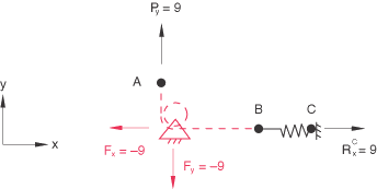
The global force balance can also be incomplete. This is demonstrated in Figure 3, where a pulley connection between nodes A and B is represented by the linear constraint equation $u_{y}^{A} - u_{x}^{B} = 0$ . The constraint forces at the pulley, $F_{x}$ and $F_{y}$ , are not included in the reaction force output, producing incomplete global force balances in both the X- and Y-directions.

Obtaining the Constraint Force

The linear constraint generates constraint forces at all the degrees of freedom involved in the equation. For a given constraint equation these forces are proportional to their respective coefficients. To find the constraint forces, introduce a node Z that is not attached to any element in the model; rewrite the constraint equation as

A_{1} u_{i}^{P} + A_{2} u_{j}^{Q} + \dots + A_{N} u_{k}^{R} - A_{1} {\hat{u}}_{m}^{Z} = 0;

and specify a zero displacement boundary condition at degree of freedom m of node Z. The reaction force obtained at node Z will be equal to the constraint force acting at node P in degree of freedom i. The constraint force in any term with coefficient $A_{K}$ in the constraint equation is obtained by multiplying the constraint force at node P in degree of freedom i with the ratio $A_{K} / A_{1}$ . For example, if the equation is

u_{3}^{5} - u_{3}^{6} = 0

and the forces in the constraint are needed, the equation can be rewritten as

u_{3}^{5} - u_{3}^{6} - u_{3}^{1000} = 0,

where node 1000 is the fixed “dummy” node. Since the coefficient of $u_{3}^{5}$ is the opposite of the coefficient of $u_{3}^{1000}$ , the constraint force at node 5 is the same as the reaction force at node 1000. Since the coefficient of $u_{3}^{6}$ is the same as the coefficient of $u_{3}^{1000}$ , the constraint force at node 6 is the opposite of the reaction force at node 1000.

Defining a Constraint in a Deformed State

You might want to impose an equation starting at a certain point in the analysis:

A_{1} Δ u_{i}^{P} + A_{2} Δ u_{j}^{Q} + \dots + A_{N} Δ u_{k}^{R} = 0,

where $Δ u$ represents the change in displacement after time $t_{0}$ . The equation can be rewritten as

A_{1} u_{i}^{P} + A_{2} u_{j}^{Q} + \dots + A_{N} u_{k}^{R} - {\hat{u}}_{m}^{Z} = 0,

where, again, node Z is not attached to any element in the model. Prior to time $t_{0}$ (which is assumed to be at the end of a step), degree of freedom m of node Z is left unrestrained. After time $t_{0}$ further changes in ${\hat{u}}_{m}^{Z}$ are restrained in Abaqus/Standard by applying a boundary condition fixing the degree of freedom at its current values at the start of the step.

Reading the Data from an Alternate Input File

The input for a linear constraint equation can be contained in a separate input file.