Connector Functions for Coupled Behavior

This section describes how to define two special functions used to specify complex coupled behavior for a connector element in Abaqus: derived components and potentials.

Connector derived components are user-specified component definitions based on a function of intrinsic (1 through 6) connector components of relative motion. They can be used:

  • to specify the friction-generating normal force in connectors as a complex combination of connector forces and moments, and

  • as an intermediate result in a connector potential function.

Connector potentials are user-defined functions of intrinsic components of relative motion or derived components. These functions can be quadratic, elliptical, or maximum norms. They can be used to define:

  • the yield function for connector coupled plasticity when several available components of relative motion are involved simultaneously,

  • the potential function for coupled user-defined friction when the slip direction is not aligned with an available component of relative motion,

  • a magnitude measure as a coupled function of connector forces or motions used to detect the initiation of damage in the connector, and

  • an effective motion measure as a coupled function of connector motions to drive damage evolution in the connector.

This page discusses:

Defining Derived Components for Connector Elements

The definition of coupled behavior in connector elements beyond simple linear elasticity or damping often requires the definition of a resultant force involving several intrinsic (1 through 6) components or the definition of a “direction” not aligned with any of the intrinsic components. These user-defined resultants or directions are called derived components. The forces and motions associated with these derived components are functions of the forces and motions in the intrinsic relative components of motion in the connector element.

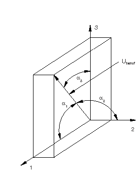
Consider the case of a SLOT connector for which frictional effects (see Connector Friction Behavior) are defined in the only available component of relative motion (the 1-direction). The two constraints enforced by this connection type will produce two reaction forces (f2 and f3), as shown in Figure 1. Both forces generate friction in the 1-direction in a coupled fashion.

Resultant contact force in a SLOT connector.

A reasonable estimate for the resulting contact force is

F derived contact = g ( f ) = f 2 2 + f 3 2 ,

where f is the collection of connector forces and moments in the intrinsic components. The function g(f) can be specified as a derived component.

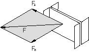
Resultant forces that can be defined as derived components may take more complicated forms. Consider a BUSHING connection type for which a tensile (Mode I) damage mechanism with failure is to be specified in the 1-direction. You may wish to include the effects of the axial force f1 and of the resultant of the “flexural” moments m2 and m3 in defining an overall resultant force in the axial direction upon which damage initiation (and failure) can be triggered, as shown in Figure 2.

Resultant axial force in a BUSHING connector.

One choice would be to define the resultant axial force as

F derived axial = g ( f ) = | f 1 | + α ( m 2 2 + m 3 2 ) ,

where α is a geometric factor relating translations to rotations with units of one over length. The function g(f) can be specified as a derived component.

A derived component can also be interpreted as a user-specified direction that is not aligned with the connector component directions. For example, if the motion-based damage with failure criterion in a CARTESIAN connection with elastic behavior does not align with the intrinsic component directions, the damage criterion can be defined in terms of a derived component representing a different direction, as shown in Figure 3.

User-defined direction in a CARTESIAN connector.

One possible choice for the direction could be

u derived transf = g ( u ) = a 1 u 1 + a 2 u 2 + a 3 u 3 ,

where u is the collection of connector relative motions in the components and a1, a2, and a3 can be interpreted as direction cosines (cos(α1), cos(α2), cos(α3)). The function g(u) can be specified as a derived component.

Functional Form of the Derived Component

The functional form of a derived component (g) in Abaqus is quite general; you specify its exact form. The derived component is specified as a sum of terms

g ( c ) = i = 1 N T T i ( c ) ,

where c is a generic name for the connector intrinsic component values (such as forces, f, or motions, u), Ti is the ith term in the sum, and NT is the number of terms. The appropriate component values for c are selected depending on the context in which the derived component is used. Ti is also a summation of several contributions and can take one of the following three forms:

  • a norm (gN-type)

    T i ( c ) = s i j = 1 N c ( α j c j ) 2 ,                 or
  • a direct sum (gS-type)

    T i ( c ) = s i j = 1 N c α j c j ,                 or
  • a Macauley sum (gM-type)

    T i ( c ) = s i j = 1 N c < α j c j > ,

where s i is the term's sign (plus or minus), α j are scaling factors, c j is the j th component of c , and < X > is the Macauley bracket ( X = 0      if      X 0      and = X      if      X > 0 ). In general, the units of the scaling factors α j depend on the context. In most cases they are either dimensionless, have units of length, or have units of one over length. The scaling factors should be chosen such that all the terms in the resulting derived component have the same units, and these units must be consistent with the use of the derived component later on in a connector potential or connector contact force.

Defining a Derived Component with Only One Term (NT = 1)

Connector derived components are identified by the names given to them. If one term (T1) is sufficient to define the derived component g, specify only one connector derived component definition.

Defining a Derived Component Containing Multiple Terms (NT > 1)

If several terms (T1, T2, etc.) are needed in the overall definition of the derived component g, you must define the individual terms.

Specifying a Term in the Derived Component as a Norm

By default, a derived component term is computed as the square root of the sum of the squares of each intrinsic component contribution. If the term has only one contribution (NC=1), the norm has the same meaning as the absolute value.

Specifying a Term in the Derived Component as a Direct Sum

Alternatively, you can choose to compute a derived component term as the direct sum of the intrinsic component contributions.

Specifying a Term in the Derived Component as a Macauley Sum

Alternatively, you can choose to compute a derived component term as the Macauley sum of the intrinsic component contributions.

Specifying the Sign of a Term

You can specify whether the sign of a derived component term should be positive or negative.

Requirements for Constructing a Derived Component Used in Plasticity or Friction Definitions

When a derived component is used to construct the yield function for a plasticity or friction definition, the following simple requirements must be satisfied:

  • All NT terms of a derived component must be of a compatible type (see Functional Form of the Derived Component); norm-type terms (gN-type) cannot be mixed with direct sum-type terms (gS-type) in the same derived component definition but can be mixed with Macauley sum-type terms (gM-type).

  • If all NT terms are norm-type terms, the sign of each term must be positive (the default).

If NT is greater than 1, the associated functions (potentials) in which the derived component is used may become non-smooth. More precisely, the normal to the hyper-surface defined by the potential may experience sudden changes in direction at certain locations. In these cases, Abaqus will automatically smooth-out the defined functions by slightly changing the derived component functional definition. These changes should be transparent to the user as the results of the analysis will change only by a small margin.

Example: Spot Weld

The spot weld shown in Figure 4 is subjected to loading in the F-direction.

Loading of a spot weld connection.

The connector chosen to model the spot weld has six available components of relative motion: three translations (components 1–3) and three rotations (components 4–6). You have chosen this connection type because you are modeling a general deformation state. However, you would like to define inelastic behavior in the connection in terms of a normal and a shear force, as shown in Figure 5, since experimental data are available in this format.

Spot weld connection: derived component definitions.

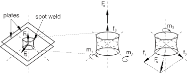
Therefore, you want to derive the normal and shear components of the force, for example, as follows:

F n = g n ( f ) = < f 3 > + ( 1 / r n ) m 1 2 + m 2 2 ,
F s = g s ( f ) = ( 1 / r s ) | m 3 | + f 1 2 + f 2 2 .

In these equations rn and rs have units of length; their interpretation is relatively straightforward if you consider the spot weld as a short beam with the axis along the spot weld axis (3-direction). If the average cross-section area of the spot weld is A and the beam's second moment of inertia about one of the in-plane axes is I11 (or I22), rn can be interpreted as the square root of the ratio I11/A (or I22/A). Furthermore, if the cross-section is considered to be circular, rn becomes equal to a fraction of the spot weld radius. In all cases rs can be taken to be 2rn.

The reasoning above for the interpretation of the calibration constants in the equations is only a suggestion. In general, any combination of constants that would lead to good comparisons with other results (experimental, analytical, etc.) is equally valuable.

To define Fn, you would specify the following two connector derived component definitions, each with the same name:

PARAMETER 
Ixx=30.68 
A=19.63 
rn=sqrt(Ixx/A) 
rs=2.0*rn 
orn=(1/rn) 
ors=(1/rs) 
CONNECTOR DERIVED COMPONENT, NAME=normal, OPERATOR=MACAULEY SUM 
3 
1.0 
CONNECTOR DERIVED COMPONENT, NAME=normal 
4, 5 
<orn>, <orn>

The <> symbols denote that orn is specified using a parameter definition. The normal force derived component Fn is defined as the sum of two terms, gn(f)=T1(f)+T2(f). The first connector derived component defines the first term T1=<f3>, while the second defines the second term T2=(1/rn)m12+m22.

Similarly, to define Fs, you would specify the following two connector derived component definitions for the component shear:

CONNECTOR DERIVED COMPONENT, NAME=shear 
6 
<ors> 
CONNECTOR DERIVED COMPONENT, NAME=shear 
1, 2 
1.0, 1.0

Defining Connector Potentials

Connector potentials are user-defined mathematical functions that represent yield surfaces, limiting surfaces, or magnitude measures in the space spanned by the components of relative motion in the connector. The functions can be quadratic, general elliptical, or maximum norms. The connector potential does not define a connector behavior by itself; instead, it is used to define the following coupled connector behaviors:

  • friction,

  • plasticity, or

  • damage.

Consider the case of a SLIDE-PLANE connection in which frictional sliding occurs in the connection plane, as shown in Figure 6.

Friction in the SLIDE-PLANE connection.

The function governing the stick-slip frictional behavior (see Connector Friction Behavior) can be written as

ϕ f r i c ( f ) = P ( f ) - μ F N ,

where P(f) is the connector potential defining the pseudo-yield function (the magnitude of the frictional tangential tractions in the connector in a direction tangent to the connection plane on which contact occurs), FN is the friction-producing normal (contact) force, and μ is the friction coefficient. Frictional stick occurs if ϕfric<0, and sliding occurs if ϕfric=0. In this case the potential can be defined as the magnitude of the frictional tangential tractions,

P ( f ) = f 2 2 + f 3 2 .

Connector potentials can also be useful in defining connector damage with a force-based coupled damage initiation criterion. For example, in a connection type with six available components of relative motion you could define a potential

P ( f ) = ( f 1 α 1 ) 2 + ( f 2 α 2 ) 2 + ( f 3 α 3 ) 2 + ( m 1 β 1 ) 2 + ( m 2 β 2 ) 2 + ( m 3 β 3 ) 2 .

Damage (with failure) can be initiated when the value of the potential P is greater than a user-specified limiting value (usually 1.0). The units of the α and β coefficients must be consistent with the units of the final product. For example, if the intended units of P(f) are newtons, the α coefficients are dimensionless while the β coefficients have units of length.

Connector potentials can take more complicated forms. Assume that coupled plasticity is to be defined in a spot weld, in which case a plastic yield criterion can be defined as

ϕ p l a s ( f ) = P ( f ) - F 0 ,

where P(f) is the connector potential defining the yield function and F0 is the yield force/moment. The potential could be defined as

P ( f ) = [ ( m a x ( F n , 0 ) R n ) β + ( | F s | R s ) β ] 1 / β ,

where Fn and Fs could be the named derived components normal and shear defined in the example in Defining Derived Components for Connector Elements above. If F0 has units of force and Fn and Fs also have units of force, Rn and Rs are dimensionless.

Functional Form of the Potential

The functional form of the potential P in Abaqus is quite general; you specify its exact form. The potential is specified as one of the following direct functions of several contributions:

a quadratic form
P ( c ) = ( i = 1 N p s i P i ( c ) 2 ) 1 2 ,
a general elliptical form
P ( c ) = ( i = 1 N p s i P i ( c ) α i ) 1 β ,     or
a maximum form
P ( c ) = max i = 1 N p s i P i ( c ) ,

where c is a generic name for the connector intrinsic component values (such as forces, f, or motions, u), Pi is the ith contribution to the potential, Np is the number of contributions, β and αi are positive numbers (defaults β= 2.0, αi=β), and si is the overall sign of the contribution (1.0 – default, or −1.0). The appropriate component values for c are selected depending on the context in which the potential is used in. The positive exponents (αi, β) and the sign si should be chosen such that the contribution Pi yields a real number.

Pi is a direct function of either an intrinsic connector component (1 through 6) or a derived connector component. Since derived components are ultimately a function of intrinsic components (see Defining Derived Components for Connector Elements), the contribution Pi is ultimately a function of c. Pi is defined as

P i ( c ) = H i ( X i ( c ) )          ( no      sum      on      i ) ,
X i ( c ) = E i ( c ) - a i R i ,

where

H i ( X )

is the function used to generate the contribution:

  • absolute value (default, |X|),

  • Macauley bracket ( X = 0      if      X 0      and = X      if      X > 0 ), or

  • identity (X);

E i

is the value of the identified component (intrinsic or derived);

a i

is a shift factor (default 0.0); and

R i

is a scaling factor (default 1.0).

The function Hi(X) can be the identity function only if αi=β=1.0. The units of the various coefficients in the equations above depend on the context in which the potential is used. In most cases the coefficients in the equations above are either dimensionless, have units of length, or have units of one over length. In all cases you must be careful in defining potentials for which the units are consistent.

Defining the Potential as a Quadratic or General Elliptical Form

To define a general elliptical form of the potential, you must specify the inverse of the overall exponent, β. You can also define the exponents αi if they are different from the default value, which is the specified value of β.

Defining the Potential as a Maximum Form

Alternatively, you can define the potential as a maximum form.

Requirements for Constructing a Potential Used in Plasticity or Friction Definitions

The connector potential, P(c), can be defined using intrinsic components of relative motion, derived components, or both. A particular contribution to the potential may be one of the following two types:

When used in the context of connector plasticity or connector friction, the potential must be constructed such that the following requirements are satisfied:

  • All Np contributions to the potential must be of the same type. Mixed PN and PS contributions are not allowed in the same potential definition.

  • If all NT terms are PN-type terms, the sign of each term must be positive (the default).

  • The positive numbers β and αi cannot be smaller than 1.0 and must be equal (the default).

Example: Spot Weld

Referring to the spot weld shown in Figure 5 and the yield function ϕplas(F) defined above, you would define this potential using the derived components normal and shear with the following input:

PARAMETER 
Rn=0.02 
Rs=0.05 
β=1.5 
CONNECTOR POTENTIAL, EXPONENT=β 
normal, Rn, , MACAULEY 
shear, Rs, , ABS

Output

The Abaqus/Explicit output variables available for connectors are listed in Abaqus/Explicit Output Variable Identifiers. The following variables (available only in Abaqus/Explicit ) are of particular interest when defining connector functions for coupled behavior:

CDERF

Connector derived force/moment with the connector derived component name appended to the output variable. If the connector derived component is used with connector plasticity, connector friction, and connector damage initiation (type force), the derived components used to form the potential represent forces and this quantity is available for both field and history output. If connector friction is used with contact force, the derived components are not used to form a potential, and the derived force is in fact the connector normal forceCNF (which is available for connector history output.)

CDERU

Connector derived displacement/rotation with the connector derived component name appended to the output variable. If the connector derived component is used with motion type for the connector damage initiation and connector damage evolution, the derived components to form the potential represent displacements and this quantity is available for both field and history output.