Contact Cohesive Behavior

The capability described in this section can be used to model a bonded interface, with or without the possibility of damage and failure of the bond, and to model regular contact behavior where the interface is not bonded. This capability has similarities to other features that could be considered for a bonded interface, including cohesive elements (see About Cohesive Elements). Cohesive contact behavior is typically easier to define than modeling the interface using cohesive elements and allows simulation of a wider range of cohesive interactions, such as two sticky surfaces coming into contact during an analysis.

Contact cohesive behavior is primarily intended for situations in which the interface thickness is negligibly small. If the interface adhesive layer has a finite thickness and macroscopic properties (such as stiffness and strength) of the adhesive material are available, it may be more appropriate to model the response using conventional cohesive elements (see Defining the Constitutive Response of Cohesive Elements Using a Continuum Approach).

In Abaqus/Explicit the surface-based cohesive behavior framework can also be used to model crack propagation in initially partially bonded surfaces via linear elastic fracture mechanics principles (LEFM) as implemented using the Virtual Crack Closure Technique (VCCT).

Contact cohesive behavior:

is defined as a surface interaction property;
can be used to model the delamination at interfaces directly in terms of traction versus separation;
can be used to model “sticky” contact (i.e., surfaces or parts of surfaces that are not initially in contact may bond on coming into contact; subsequently the bond may damage and fail);
can be restricted to surface regions that are initially in contact;
allows specification of cohesive data such as the fracture energy as a function of the ratio of normal to shear displacements (mode mix) at the interface;
assumes a linear elastic traction-separation law prior to damage;
assumes that failure of the cohesive bond is characterized by progressive degradation of the cohesive stiffness, which is driven by a damage process (in Abaqus/Explicit brittle fracture can also be modeled using a VCCT fracture crierion);
allows specification of postfailure cohesive behavior if failed nodes re-enter contact;
is implemented within the general contact algorithmic framework in Abaqus/Standard and Abaqus/Explicit and within the contact pair framework in Abaqus/Standard;
is enforced with the surface-to-surface, edge-to-surface, edge-to-edge, and vertex-to-surface contact formulations for general contact in Abaqus/Standard;
is enforced only for node-to-face contact interactions in Abaqus/Explicit and is not available for edge-to-edge and node-to-analytical rigid surface contact interactions;
is enforced for the node-to-surface contact formulation for contact pairs in Abaqus/Standard and is not available for the finite-sliding, surface-to-surface contact formulation for contact pairs in Abaqus/Standard;
can be used as an alternative to rough friction surface interactions, the no separation contact relationship, or a combined no separation and rough friction behavior within the general contact framework;
is an alternative way to tie surfaces; and
cannot be used in a coupled Eulerian-Lagrangian analysis in Abaqus/Explicit.

This page discusses:

Common Usages of Cohesive Contact Behavior
High-Level Comparison of Cohesive-Element and Cohesive-Contact Approaches
Specifying Cohesive Interface "Material" Behavior within a Surface Interaction Property Definition
Initial Cohesive Contact State
Limiting Cohesive Bonding to Original Contact Constraints
Cohesive Rebonding upon Repeated Contact
Limiting Cohesive Bonding to First Contact Constraints
Main and Secondary Roles and Contact Formulations Associated with Cohesive Interactions
Linear Elastic Traction-Separation Behavior
Damage Modeling
Damage Initiation
Damage Evolution
Viscous Regularization in Abaqus/Standard
Virtual Crack Closure Technique in Abaqus/Explicit
Output
References

Common Usages of Cohesive Contact Behavior

Cohesive contact can be used in a variety of workflows. Cohesive contact behavior often is one of many possible approaches to modeling interface behavior. Common usages of cohesive contact include:

Modeling a permanently bonded interface.
Modeling a bonded interface in which the bond may damage and fail.
Approximating interface behavior in a simplified form while a model is being built (and other aspects of the model are being refined).

These usages are discuss in more detail below.

Modeling a Permanently Bonded Interface

In it simplest form, cohesive contact can be used as an alternative to surface-based tie constraints (which are discussed in Mesh Tie Constraints) or other modeling methods. There is no need to specify stiffness or damage properties of the contact cohesive behavior in this case; you can allow Abaqus to assign default interfacial stiffness components. Bonded regions remain bonded throughout a simulation if cohesive damage characteristics are not specified. Unlike surface-based tie constraints, cohesive contact will not constrain rotational degrees of freedom.

Modeling a permanently bonded interface as a type of contact behavior rather than as a surface-based tie constraint has the following advantages:

Enables contact output variables to be used to evaluate interface stresses and other quantities.
Enables numerical softening to be introduced in the constraint enforcement, which avoids the potential for numerical issues associated with overconstraints where different types of strictly enforced "hard" constraints overlap.
Optionally, allows a specific interface stiffness representative of physical behavior to be specified.

Permanent cohesive bonds with default cohesive stiffness or user-specified cohesive stiffness at least as stiff as the default cohesive stiffness have the following characteristics for general contact in Abaqus/Standard:

No regular contact constraints act in parallel to cohesive contact constraints: Conditions for regular contact constraints acting in parallel to cohesive contact constraints are discussed in Interaction between Cohesive Properties and Regular Contact Properties. However, those conditions are not relevant to stiff, permanent cohesive constraints, and regular contact constraints are avoided in these cases to improve convergence behavior and performance.
Details of the cohesive contact formulation are enhanced for stiff, permanent cohesive bonds. Results for stiff cohesive bonds may differ, even prior to cohesive damage, depending on whether or not a cohesive damage evolution model is specified.

Modeling a Bonded Interface That May Fail

Specifying a damage model for the contact cohesive behavior allows for modeling of a bonded interface that may fail as a result of the loading. This modeling approach is an alternative to using cohesive elements or other element types that directly discretize the cohesive material for the simulation. Comparisons of cohesive-contact versus cohesive-element approaches are discussed below in High-Level Comparison of Cohesive-Element and Cohesive-Contact Approaches.

Approximating and Modifying Interface Behavior While a Finite Element Model Is Built

Using different interface modeling strategies across different stages of building and refining a finite element model is sometimes a good strategy for improving your efficiency. For example, during an initial stage of a model build, you may choose to model interfaces as permanently bonded to enable more focus on noninterface modeling details. You can switch to more physically representative interface behavior (such as regular contact or bonded contact with the possibility of damage and failure) in later stages of the model build. The later stages often require more care to avoid unconstrained rigid body modes and other types of static instabilities.

Analysts sometimes use surface-based tie constraints (Mesh Tie Constraints) in early stages of building a model and then switch to contact specifications as the model becomes more mature. An alternative is to specify cohesive contact behavior with a permanently bonded interface and default stiffness in the early stages, and then reassign a more realistic contact behavior as the model becomes more mature. This alternative of reassigning the contact behavior as the model matures, rather than switching from a constraint option to a contact option during the model evolution, may result in greater consistency across different stages of the model build.

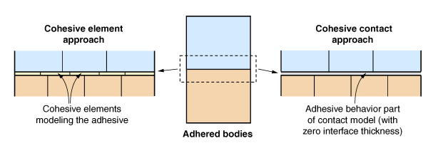
High-Level Comparison of Cohesive-Element and Cohesive-Contact Approaches

Figure 1 provides a high-level comparison of the cohesive-element and cohesive-contact modeling approaches. Both of these approaches are viable for many modeling situations.

The formulae and laws that govern cohesive constitutive behavior are very similar for cohesive contact and cohesive elements. The similarities extend to the linear elastic traction-separation model, damage initiation criteria, and damage evolution laws. Constitutive behavior details for contact cohesive behavior are discussed later in this section, starting with Linear Elastic Traction-Separation Behavior. Constitutive behavior details for cohesive element are discussed in Defining the Constitutive Response of Cohesive Elements Using a Traction-Separation Description.

It is important to recognize differences between the cohesive-contact and cohesive-element approaches, including the aspects discussed below.

No Cohesive Contact Thickness

Cohesive material thickness cannot be introduced as a characteristic for cohesive contact but can be for cohesive elements. Surface thickness can be modified (Assigning Surface Properties) to account for cohesive material thickness. Since thickness effects are not considered for a cohesive property, material definitions used to describe traction-separation response for cohesive elements with thickness effects may not be directly reusable for cohesive contact.

Tangential Refinement of the Interface

Constitutive calculations are evaluated for cohesive contact and cohesive elements at the following locations:

For cohesive elements, constitutive calculations are calculated at the material points of the elements.
For cohesive contact, constitutive calculations are calculated for individual contact constraints. The number of potential contact constraints is approximately equal to the number of nodes acting as secondary nodes.

Modeling with cohesive elements allows the possibility of different tangential mesh refinement for cohesive elements as compared to the mesh refinement of the adjacent bodies. Use of a more refined mesh for the cohesive elements may improve the resolution of spatial variations in the cohesive response, independent, to a degree, of the mesh refinement of the adjacent bodies. The cohesive element example in Figure 1 shows a slightly more refined mesh for the cohesive elements than the adjacent bodies.

For the cohesive contact modeling approach, cohesive calculations are computed at contact constraint locations, which are primarily associated with secondary nodes. The more refined surface of an interaction typically acts as the secondary surface. Therefore, the resolution of spatial variations in the cohesive response is usually primarily associated with whichever adjacent body has the more refined surface.

Interaction between Cohesive Properties and Regular Contact Properties

"Regular" contact behavior is automatically in effect if the cohesive contact bond becomes fully damaged. Cohesive elements do not have an analogous behavior in this regard unless contact is defined between surfaces of the adhered parts in addition to having cohesive elements defined between the adhered parts. A surface interaction property definition containing cohesive specifications will also include noncohesive, mechanical contact specifications, such as discussed in Contact Pressure-Overclosure Relationships and Frictional Behavior.

"Regular" contact-behavior aspects are sometimes partially in effect even before the cohesive has failed, as described below:

Normal-direction behavior: The noncohesive contact pressure-overclosure relationship (see Contact Pressure-Overclosure Relationships) is in effect while the contact pressure is positive, regardless of whether cohesive behavior is specified and the amount of cohesive damage accumulated except for stiff, permanent cohesive cohesive behavior. No regular contact constraints act in parallel to cohesive contact constraints for stiff, permanent cohesive behavior.
Tangential behavior: If cohesive bonding at a particular interface location is active and undamaged, the resistance to tangential motion is governed by the cohesive behavior only. Once cohesive damage starts to accumulate at a particular location of the interface, the interface shear stress has contributions from the cohesive model and the friction model. The contribution from the friction model is weighted by the scalar damage variable of the cohesive behavior (see Damage Evolution). When the cohesive bond is fully damaged (failed), the only contribution to the interface shear stress is from the friction model.

Nonmechanical interactions are ignored when surface-based cohesive behavior is defined.

Interface Versus Element Quantities

The table below compares how various simulation operations associated with cohesive modeling can be performed with the cohesive contact and cohesive element modeling approaches.


Simulation operation	Cohesive contact	Cohesive elements
Defining where a cohesive region is located	Interaction property assignment (based on surface pairings)	Including cohesive elements (and nodes) in the model
Defining cohesive damage model and other aspects of cohesive constitutive behavior	Interaction property specification	Material property specification
Studying results for stretching and shearing of a cohesive material	Contact opening and sliding distance output	Element strain output
Studying results for stresses within a cohesive material	Contact stresses output for normal and tangent directions	Element stress output

Specifying Cohesive Interface "Material" Behavior within a Surface Interaction Property Definition

Cohesive interface "material" behavior is defined as part of a surface interaction property. Surface interaction properties are assigned to contact interactions as discussed in Defining the Contact Property Model. Cohesive interface behavior includes stiffness characteristics associated with the bonded interface and characteristics governing any cohesive damage. Bonded-interface stiffness characteristics are assigned by default if these stiffness characteristics are not specified explicitly. The magnitudes of these default stiffness characteristics are similar to the magnitude of the default contact penalty stiffness. A damage model is not included in the cohesive material behavior unless damage characteristics are specified explicitly as part of the damage behavior definition.

Initial Cohesive Contact State

The initial contact status as a function of position along a cohesive contact interface can fundamentally affect simulation results. Consider the example shown in Figure 2. The intent for this example is that the block is initially touching the wall with the cohesive status initialized to bonded. However, a small, unintended initial gap exists between the block and the wall in the initial configuration, so the contact status is initialized to "opened" or "inactive," and the cohesive status is initialized to unbonded by default. If there is no initial cohesive bonding in this example, the applied force will push the block away from the wall or perhaps, in a static analysis, a numerical issue will be reported by Abaqus/Standard due to unconstrained rigid-body motion of the block. User controls associated with the initial contact status (see Contact Initialization for General Contact in Abaqus/Standard, Contact Initialization for Contact Pairs in Abaqus/Standard, and Contact Initialization for General Contact in Abaqus/Explicit) can be used to ensure that the contact status will be properly initialized over various regions of an interface, such that interface stresses associated with cohesive contact will counter the applied force. Most user controls associated with the initial contact status are not specific to cohesive contact behavior.

Consider the example shown in Figure 3, in which the cohesive status is intended to be initialized to bonded over much of the interface but should be initialized to unbonded over a specific portion of the interface. The desired initialization can be achieved by assigning zero initial clearance to the portion of the interface that should be initially bonded and very small positive initial clearance to the portion of the interface that should not be initially bonded, such as shown in the Abaqus/Standard input file example below.

CONTACT INITIALIZATION DATA, NAME=TOUCHING, INITIAL CLEARANCE=0.0, SEARCH ABOVE=0.1
CONTACT INITIALIZATION DATA, NAME=SMALL_GAP, INITIAL CLEARANCE=1.E-7, SEARCH ABOVE=0.1
…
CONTACT
…
CONTACT INITIALIZATION ASSIGNMENT
BLOCK_SURF_BONDED_REGION, RIGID_SURF, TOUCHING
BLOCK_SURF_UNBONDED_REGION, RIGID_SURF, SMALL_GAP

Limiting Cohesive Bonding to Original Contact Constraints

The most common usage of cohesive contact is for situations in which cohesive bonds exist at the beginning of a simulation. By default, Abaqus limits cohesive bonds to those that exist at the beginning of a simulation.

Limiting Cohesive Bonding to Subset of Original Contact Constraints

For contact pairs in Abaqus/Standard you can specify as part of the cohesive behavior definition that only a subset of initially active contact constraints should have cohesive bonds. Initial strain-free adjustments to positions of secondary nodes will be made, if necessary, to ensure they are initially in contact with the main surface. Similar behavior can be achieved with general contact by selectively assigning initialization controls to control which regions of the interface are initially in contact and limiting cohesive behavior to initially active contact constraints (see Initial Cohesive Contact State).

Cohesive Rebonding upon Repeated Contact

In some situations it is desirable to allow cohesive rebonding each time contact is established, even for secondary nodes previously involved in cohesive contact that have fully damaged and debonded. For such situations, you can indicate that cohesive rebonding can repeatedly occur at the same interface location.

Cohesive Rebonding upon Repeated Contact Limited to Locations of Initial Cohesive Bonds

General contact in Abaqus/Explicit and contact pairs in Abaqus/Standard allow cohesive bonding to be limited to originally active contact constraints with only these secondary nodes to be eligible to rebond upon subsequent contact, and contact pairs in Abaqus/Standard allow this behavior for a subset of initially active contact constraints.

Limiting Cohesive Bonding to First Contact Constraints

It is sometimes desirable to establish cohesive bonds for initial contact constraints plus the first time an initially not-in-contact region comes into contact during a simulation. General contact in Abaqus/Explicit and contact pairs in Abaqus/Standard optionally support each secondary node associated with interactions that are assigned a cohesive property to become bonded once (either initially or during a simulation). Simulation results with this option can be highly sensitive to the assignment of secondary and main roles since the check for prior cohesive bonds at a location is done only for nodes acting as secondary nodes. General contact in Abaqus/Standard allows cohesive behavior to be limited to initial contact constraints (see Limiting Cohesive Bonding to Original Contact Constraints) and allows cohesive behavior for all new contact constraints (see Cohesive Rebonding upon Repeated Contact) but does not support limiting cohesive behavior to first contact constraints.

When cohesive contact behavior applies to contact that develops after the start of the simulation, cohesive effects are activated one increment after the contact constraint becomes active.

Main and Secondary Roles and Contact Formulations Associated with Cohesive Interactions

Interactions assigned a cohesive surface interaction property are modeled with pure main-secondary roles in the contact formulation. The main and secondary roles are established as follows:

General contact in Abaqus/Standard: main and secondary roles for interactions associated with cohesive behavior are the same as for other types of contact behavior (see Main and Secondary Surface Roles of a Contact Formulation).
General contact in Abaqus/Explicit: main and secondary roles for interactions associated with cohesive behavior follow the convention that the first surface specified in a contact property assignment involving cohesive behavior is treated as a secondary surface and the second surface is treated as its corresponding main surface.
Contact pairs in Abaqus/Standard: main and secondary roles are defined by the usual conventions associated with defining a contact pair.

Linear Elastic Traction-Separation Behavior

The available traction-separation model in Abaqus assumes initially linear elastic behavior (see Defining Elasticity in Terms of Tractions and Separations for Cohesive Elements) followed by the initiation and evolution of damage. The elastic behavior is written in terms of an elastic constitutive matrix that relates the normal and shear stresses to the normal and shear separations across the interface.

The nominal traction stress vector, $t$ , consists of three components (two components in two-dimensional problems): $t_{n}$ , $t_{s}$ , and (in three-dimensional problems) $t_{t}$ , which represent the normal (along the local 3-direction in three dimensions and along the local 2-direction in two dimensions) and the two shear tractions (along the local 1- and 2-directions in three dimensions and along the local 1-direction in two dimensions), respectively. The corresponding separations are denoted by $δ_{n}$ , $δ_{s}$ , and $δ_{t}$ . The elastic behavior can then be written as

t = {\begin{matrix} t_{n} \\ t_{s} \\ t_{t} \end{matrix}} = [\begin{matrix} K_{n n} & K_{n s} & K_{n t} \\ K_{n s} & K_{s s} & K_{s t} \\ K_{n t} & K_{s t} & K_{t t} \end{matrix}] {\begin{matrix} δ_{n} \\ δ_{s} \\ δ_{t} \end{matrix}} = K δ .

Uncoupled Traction-Separation Behavior

The simplest specification of cohesive behavior generates contact penalties that enforce the cohesive constraint in both normal and tangential directions. By default, the normal and tangential stiffness components will not be coupled: pure normal separation by itself does not give rise to cohesive forces in the shear directions, and pure shear slip with zero normal separation does not give rise to any cohesive forces in the normal direction.

For uncoupled traction-separation behavior, the terms $K_{n n}$ , $K_{s s}$ , and $K_{t t}$ must be defined, as well as any dependencies on temperature or field variables. If these terms are not defined, Abaqus uses default contact penalties to model the traction-separation behavior.

Coupled Traction-Separation Behavior

In its full generality, the elasticity matrix provides fully coupled behavior between all components of the traction vector and separation vector and can depend on temperature and/or field variables. All terms in the matrix must be defined for coupled traction-separation behavior.

Cohesive Behavior in the Normal or Shear Direction Only

To restrict the cohesive constraint to act along the contact normal direction only, define uncoupled cohesive behavior and specify zero values for the shear stiffness components, $K_{s s}$ and $K_{t t}$ . Alternatively, if only tangential cohesive constraints are to be enforced, the normal stiffness term, $K_{n n}$ , can be set to zero, in which case the normal “separations” will not be constrained. Normal compressive forces are resisted as per the usual contact behavior.

Damage Modeling

Damage modeling allows you to simulate the degradation and eventual failure of the bond between two cohesive surfaces. The failure mechanism consists of two ingredients: a damage initiation criterion and a damage evolution law. The initial response is assumed to be linear as discussed above. However, once a damage initiation criterion is met, damage can occur according to a user-defined damage evolution law. 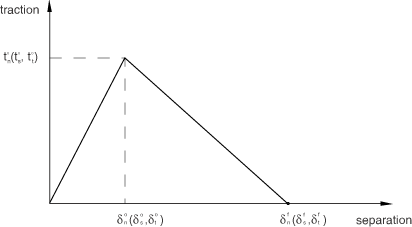Figure 4 shows a typical traction-separation response with a failure mechanism. If the damage initiation criterion is specified without a corresponding damage evolution model, Abaqus evaluates the damage initiation criterion for output purposes only; there is no effect on the response of the cohesive surfaces (i.e., no damage will occur). Cohesive surfaces do not undergo damage under pure compression.

Damage of the traction-separation response for cohesive surfaces is defined within the same general framework used for conventional materials (see About Progressive Damage and Failure), except the damage behavior is specified as part of the interaction properties for the surfaces. Multiple damage response mechanisms are not available for cohesive surfaces: cohesive surfaces can have only one damage initiation criterion and only one damage evolution law.

Damage Initiation

Damage initiation refers to the beginning of degradation of the cohesive response at a contact point. The process of degradation begins when the contact stresses and/or contact separations satisfy certain damage initiation criteria that you specify. Several damage initiation criteria are available and are discussed below.

Each damage initiation criterion also has an output variable associated with it to indicate whether the criterion is met. A value of 1 or higher indicates that the initiation criterion has been met. Damage initiation criteria that do not have an associated evolution law affect only output. Thus, you can use these criteria to evaluate the propensity of the material to undergo damage without actually modeling the damage process (i.e., without actually specifying damage evolution).

In the discussion below, $t_{n}^{o}$ , $t_{s}^{o}$ , and $t_{t}^{o}$ represent the peak values of the contact stress when the separation is either purely normal to the interface or purely in the first or the second shear direction, respectively. Likewise, $δ_{n}^{o}$ , $δ_{s}^{o}$ , and $δ_{t}^{o}$ represent the peak values of the contact separation, when the separation is either purely along the contact normal or purely in the first or the second shear direction, respectively. The symbol $⟨ ⟩$ used in the discussion below represents the Macaulay bracket with the usual interpretation. The Macaulay brackets are used to signify that a purely compressive displacement (i.e., a contact penetration) or a purely compressive stress state does not initiate damage.

Maximum Stress Criterion

Damage is assumed to initiate when the maximum contact stress ratio (as defined in the expression below) reaches a value of one. This criterion can be represented as

\max {\frac{⟨ t_{n} ⟩}{t_{n}^{o}}, \frac{t_{s}}{t_{s}^{o}}, \frac{t_{t}}{t_{t}^{o}}} = 1.

Maximum Separation Criterion

Damage is assumed to initiate when the maximum separation ratio (as defined in the expression below) reaches a value of one. This criterion can be represented as

\max {\frac{⟨ δ_{n} ⟩}{δ_{n}^{o}}, \frac{δ_{s}}{δ_{s}^{o}}, \frac{δ_{t}}{δ_{t}^{o}}} = 1.

Quadratic Stress Criterion

Damage is assumed to initiate when a quadratic interaction function involving the contact stress ratios (as defined in the expression below) reaches a value of one. This criterion can be represented as

{\frac{⟨ t_{n} ⟩}{t_{n}^{o}}}^{2} + {\frac{t_{s}}{t_{s}^{o}}}^{2} + {\frac{t_{t}}{t_{t}^{o}}}^{2} = 1.

Quadratic Separation Criterion

Damage is assumed to initiate when a quadratic interaction function involving the separation ratios (as defined in the expression below) reaches a value of one. This criterion can be represented as

{\frac{⟨ δ_{n} ⟩}{δ_{n}^{o}}}^{2} + {\frac{δ_{s}}{δ_{s}^{o}}}^{2} + {\frac{δ_{t}}{δ_{t}^{o}}}^{2} = 1.

Rate Dependency

The damage initiation criterion can be defined as a tabular function of the effective rate of separation.

Damage Evolution

The damage evolution law describes the rate at which the cohesive stiffness is degraded once the corresponding initiation criterion is reached. The general framework for describing the evolution of damage in bulk materials (as opposed to interfaces modeled using cohesive surfaces) is described in Damage Evolution and Element Removal for Ductile Metals. Conceptually, similar ideas apply for describing damage evolution in cohesive surfaces.

A scalar damage variable, D, represents the overall damage at the contact point. It initially has a value of 0. If damage evolution is modeled, D monotonically evolves from 0 to 1 upon further loading after the initiation of damage. The contact stress components are affected by the damage according to

t_{n} = {\begin{matrix} (1 - D) {\bar{t}}_{n}, & {\bar{t}}_{n} \geq 0 \\ {\bar{t}}_{n}, & otherwise (no damage to compressive
  stiffness); \end{matrix}

t_{s} = (1 - D) {\bar{t}}_{s},

t_{t} = (1 - D) {\bar{t}}_{t},

where ${\bar{t}}_{n}$ , ${\bar{t}}_{s}$ , and ${\bar{t}}_{t}$ are the contact stress components predicted by the elastic traction-separation behavior for the current separations without damage.

To describe the evolution of damage under a combination of normal and shear separations across the interface, it is useful to introduce an effective separation (Camanho and Davila, 2002) defined as

δ_{m} = \sqrt{{⟨ δ_{n} ⟩}^{2} + δ_{s}^{2} + δ_{t}^{2}} .

While this formula was originally applied to damage evolution in cohesive elements, it can be reinterpreted in terms of contact separations for cohesive surface behavior, as discussed above (see High-Level Comparison of Cohesive-Element and Cohesive-Contact Approaches).

Mixed-Mode Definition

The relative proportions of normal and shear separations at a contact point define the mode mix at the point. Abaqus uses three measures of mode mix, two that are based on energies and one that is based on tractions. You can choose one of these measures when you specify the mode dependence of the damage evolution process. Denoting by $G_{n}$ , $G_{s}$ , and $G_{t}$ the work done by the tractions and their conjugate separations in the normal, first, and second shear directions, respectively, and defining $G_{T} = G_{n} + G_{s} + G_{t}$ , the mode-mix definitions based on energies are as follows:

m_{1} = \frac{G_{n}}{G_{T}},

m_{2} = \frac{G_{s}}{G_{T}},

m_{3} = \frac{G_{t}}{G_{T}} .

Clearly, only two of the three quantities defined above are independent. It is also useful to define the quantity $G_{S} = G_{s} + G_{t}$ to denote the portion of the total work done by the shear traction and the corresponding separation components. As discussed later, Abaqus requires that you specify material properties related to damage evolution as functions of $m_{2} + m_{3} ( = G_{S} / G_{T})$ (or, equivalently, $1 - m_{1}$ ) and $m_{3} / (m_{2} + m_{3}) ( = G_{t} / G_{S})$ .

Abaqus computes the energy quantities described above either based on the current state of deformation (nonaccumulative measure of energy) or based on the deformation history (accumulative measure of energy) at an integration point. The former approach, available only in Abaqus/Standard, is useful in mixed-mode simulations where the primary energy dissipation mechanism is associated with the creation of new surfaces due to failure in the cohesive zone. Such problems are typically adequately described utilizing the methods of linear elastic fracture mechanics. The latter approach provides an alternate way of defining the mode-mix and may be useful in situations where other significant dissipation mechanisms also govern the overall structural response.

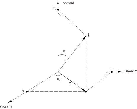
The corresponding definitions of the mode mix based on traction components are given by

ϕ_{1} = (\frac{2}{π}) \tan^{- 1} (\frac{τ}{⟨ t_{n} ⟩}),

ϕ_{2} = (\frac{2}{π}) \tan^{- 1} (\frac{t_{t}}{t_{s}}),

where $τ = \sqrt{t_{s}^{2} + t_{t}^{2}}$ is a measure of the effective shear traction. The angular measures used in the above definition (before they are normalized by the factor $2 / π$ ) are illustrated in Figure 5.

Comparison of Mixed-Mode Definitions

The mode-mix ratios defined in terms of energies and tractions can be quite different in general. The following example illustrates this point. In terms of energies a separation in the purely normal direction is one for which $G_{n} \neq 0$ and $G_{s} = G_{t} = 0$ , irrespective of the values of the normal and the shear tractions. In particular, for coupled traction-separation behavior both the normal and shear tractions may be nonzero for a purely normal separation. For this case the definition of mode mix based on energies would indicate a purely normal separation, while the definition based on tractions would suggest a mix of both normal and shear separation.

When the mode mix is defined based on accumulated energies, an artificial path-dependence may be introduced in the mixed-mode behavior that may not be consistent, for example, with predictions that are based on linear elastic fracture mechanics. Therefore, if an interface is first loaded purely in the normal deformation mode, unloaded, and subsequently loaded in a purely shear deformation mode, the mode-mix ratios based on accumulated energies at the end of the above deformation path evaluate to (assuming the shear deformation to be in the local-1 direction only) $G_{n} \neq 0$ and $G_{s} \neq 0$ . On the other hand, the mode-mix ratios based on nonaccumulated energies evaluate to $G_{n} = 0$ and $G_{s} \neq 0$ at the end of the above deformation path.

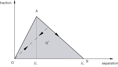
Damage Evolution Definition

There are two components to the definition of damage evolution. The first component involves specifying either the effective separation at complete failure, $δ_{m}^{f}$ , relative to the effective separation at the initiation of damage, $δ_{m}^{o}$ ; or the energy dissipated due to failure, $G^{C}$ (see Figure 6). The second component to the definition of damage evolution is the specification of the nature of the evolution of the damage variable, D, between initiation of damage and final failure. This can be done by either defining linear or exponential softening laws or specifying D directly as a tabular function of the effective separation relative to the effective separation at damage initiation. The data described above will in general be functions of the mode mix, temperature, and/or field variables.

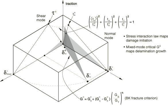
Figure 7 is a schematic representation of the dependence of damage initiation and evolution on the mode mix for a traction-separation response with isotropic shear behavior. The figure shows the traction on the vertical axis and the magnitudes of the normal and the shear separations along the two horizontal axes. The unshaded triangles in the two vertical coordinate planes represent the response under pure normal and pure shear separation, respectively. All intermediate vertical planes (that contain the vertical axis) represent the damage response under mixed-mode conditions with different mode mixes. The dependence of the damage evolution data on the mode mix can be defined either in tabular form or, in the case of an energy-based definition, analytically. The manner in which the damage evolution data are specified as a function of the mode mix is discussed later in this section.

Unloading subsequent to damage initiation is always assumed to occur linearly toward the origin of the traction-separation plane, as shown in Figure 6. Reloading subsequent to unloading also occurs along the same linear path until the softening envelope (line AB) is reached. Once the softening envelope is reached, further reloading follows this envelope as indicated by the arrow in Figure 6.

Evolution Based on Effective Separation

You specify the quantity $δ_{m}^{f} - δ_{m}^{o}$ (i.e., the effective separation at complete failure, $δ_{m}^{f}$ , relative to the effective separation at damage initiation, $δ_{m}^{o}$ , as shown in Figure 6) as a tabular function of the mode mix, temperature, and/or field variables. In addition, you also choose either a linear or an exponential softening law that defines the detailed evolution (between initiation and complete failure) of the damage variable, D, as a function of the effective separation beyond damage initiation. Alternatively, instead of using linear or exponential softening, you can specify the damage variable, D, directly as a tabular function of the effective separation after the initiation of damage, $δ_{m} - δ_{m}^{o}$ ; mode mix; temperature; and/or field variables.

Linear Damage Evolution

For linear softening (see Figure 6) Abaqus uses an evolution of the damage variable, D, that reduces (in the case of damage evolution under a constant mode mix, temperature, and field variables) to the following expression:

D = \frac{δ_{m}^{f} (δ_{m}^{\max} - δ_{m}^{o})}{δ_{m}^{\max} (δ_{m}^{f} - δ_{m}^{o})} .

In the preceding expression and in all later references, $δ_{m}^{\max}$ refers to the maximum value of the effective separation attained during the loading history. The assumption of a constant mode mix at a contact point between initiation of damage and final failure is customary for problems involving monotonic damage (or monotonic fracture).

Exponential Damage Evolution

For exponential softening (see Figure 8) Abaqus uses an evolution of the damage variable, D, that reduces (in the case of damage evolution under a constant mode mix, temperature, and field variables) to

D = 1 - {\frac{δ_{m}^{o}}{δ_{m}^{\max}}} {1 - \frac{1 - \exp (- α (\frac{δ_{m}^{\max} - δ_{m}^{o}}{δ_{m}^{f} - δ_{m}^{o}}))}{1 - \exp (- α)}} .

In the expression above $α$ is a nondimensional parameter that defines the rate of damage evolution and $\exp (x)$ is the exponential function.

Tabular Damage Evolution

For tabular softening you define the evolution of D directly in tabular form. D must be specified as a function of the effective separation relative to the effective separation at initiation, mode mix, temperature, and/or field variables.

Evolution Based on Energy

Damage evolution can be defined based on the energy that is dissipated as a result of the damage process, also called the fracture energy. The fracture energy is equal to the area under the traction-separation curve (see Figure 6). You specify the fracture energy as a property of the cohesive interaction and choose either a linear or an exponential softening behavior. Abaqus ensures that the area under the linear or the exponential damaged response is equal to the fracture energy.

The dependence of the fracture energy on the mode mix can be specified either directly in tabular form or by using analytical forms as described below. When the analytical forms are used, the mode-mix ratio is assumed to be defined in terms of energies.

Tabular Form

The simplest way to define the dependence of the fracture energy is to specify it directly as a function of the mode mix in tabular form.

Power Law Form

The dependence of the fracture energy on the mode mix can be defined based on a power law fracture criterion. The power law criterion states that failure under mixed-mode conditions is governed by a power law interaction of the energies required to cause failure in the individual (normal and two shear) modes. It is given by

{\frac{G_{n}}{G_{n}^{C}}}^{α} + {\frac{G_{s}}{G_{s}^{C}}}^{α} + {\frac{G_{t}}{G_{t}^{C}}}^{α} = 1,

The mixed-mode fracture energy $G^{C} = G_{T}$ when the above condition is satisfied. In other words,

G^{C} = 1 / {({\frac{m_{1}}{G_{n}^{C}}}^{α} + {\frac{m_{2}}{G_{s}^{C}}}^{α} + {\frac{m_{3}}{G_{t}^{C}}}^{α})}^{1 / α} .

You specify the quantities $G_{n}^{C}$ , $G_{s}^{C}$ , and $G_{t}^{C}$ , which refer to the critical fracture energies required to cause failure in the normal, the first, and the second shear directions, respectively.

Benzeggagh-Kenane (BK) Form

The Benzeggagh-Kenane fracture criterion (Benzeggagh and Kenane, 1996) is particularly useful when the critical fracture energies during separation purely along the first and the second shear directions are the same; i.e., $G_{s}^{C} = G_{t}^{C}$ . It is given by

G_{n}^{C} + (G_{s}^{C} - G_{n}^{C}) {\frac{G_{S}}{G_{T}}}^{η} = G^{C},

where $G_{S} = G_{s} + G_{t}$ , $G_{T} = G_{n} + G_{S}$ , and $η$ is a cohesive property parameter. You specify $G_{n}^{C}$ , $G_{s}^{C}$ , and $η$ .

Linear Damage Evolution

For linear softening (see Figure 6) Abaqus uses an evolution of the damage variable, D, that reduces to

D = \frac{δ_{m}^{f} (δ_{m}^{\max} - δ_{m}^{o})}{δ_{m}^{\max} (δ_{m}^{f} - δ_{m}^{o})},

where $δ_{m}^{f} = 2 G^{C} / T_{eff}^{o}$ with $T_{eff}^{o}$ as the effective traction at damage initiation. $δ_{m}^{\max}$ refers to the maximum value of the effective separation attained during the loading history.

Exponential Damage Evolution

For exponential softening Abaqus uses an evolution of the damage variable, D, that reduces to

D = \int_{δ_{m}^{o}}^{δ_{m}^{\max}} \frac{T_{eff} d δ}{G^{C} - G_{o}} .

In the expression above $T_{eff}$ and $δ$ are the effective traction and separation, respectively. $G_{o}$ is the elastic energy at damage initiation. In this case the traction might not drop immediately after damage initiation, which is different from what is seen in Figure 8.

Defining Damage Evolution Data as a Tabular Function of Mode Mix

As discussed earlier, the data defining the evolution of damage at the cohesive interface can be tabular functions of the mode mix. The manner in which this dependence must be defined in Abaqus is outlined below for mode-mix definitions based on energy and traction, respectively. In the following discussion it is assumed that the evolution is defined in terms of energy. Similar observations can also be made for evolution definitions based on effective separation.

Mode Mix Based on Energy

For an energy-based definition of mode mix, in the most general case of a three-dimensional state of separation with anisotropic shear behavior the fracture energy, $G^{C}$ , must be defined as a function of $(m_{2} + m_{3})$ and $[m_{3} / (m_{2} + m_{3})]$ . The quantity $(m_{2} + m_{3}) = G_{S} / G_{T}$ is a measure of the fraction of the total separation that is shear, while $[m_{3} / (m_{2} + m_{3})] = G_{t} / G_{S}$ is a measure of the fraction of the total shear separation that is in the second shear direction. 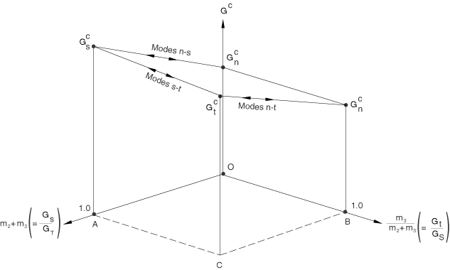Figure 9 shows a schematic of the fracture energy versus mode-mix behavior.

The limiting cases of pure normal and pure shear separations in the first and second shear directions are denoted in Figure 9 by $G_{n}^{C}$ , $G_{s}^{C}$ , and $G_{t}^{C}$ , respectively. The lines labeled “Modes n-s,” “Modes n-t,” and “Modes s-t” show the transition in behavior between the pure normal and the pure shear in the first direction, pure normal and pure shear in the second direction, and pure shears in the first and second directions, respectively. In general, $G^{C}$ must be specified as a function of $(m_{2} + m_{3})$ at various fixed values of $[m_{3} / (m_{2} + m_{3})]$ . In the discussion that follows we refer to a data set of $G^{C}$ versus $(m_{2} + m_{3})$ corresponding to a fixed $[m_{3} / (m_{2} + m_{3})]$ as a “data block.” The following guidelines are useful in defining the fracture energy as a function of the mode mix:

For a two-dimensional problem $G^{C}$ needs to be defined as a function of $m_{2}$ ( $m_{3} = 0$ in this case) only. The data column corresponding to $[m_{3} / (m_{2} + m_{3})]$ must be left blank. Hence, essentially only one “data block” is needed.
For a three-dimensional problem with isotropic shear response, the shear behavior is defined by the sum $(m_{2} + m_{3})$ and not by the individual values of $m_{2}$ and $m_{3}$ . Therefore, in this case a single “data block” (the “data block” for $[m_{3} / (m_{2} + m_{3})] = 0$ ) also suffices to define the fracture energy as a function of the mode mix.
In the most general case of three-dimensional problems with anisotropic shear behavior, several “data blocks” would be needed. As discussed earlier, each “data block” would contain $G^{C}$ versus $(m_{2} + m_{3})$ at a fixed value of $[m_{3} / (m_{2} + m_{3})]$ . In each “data block” $(m_{2} + m_{3})$ can vary between 0 and 1.0. The case $(m_{2} + m_{3}) = 0$ (the first data point in any “data block”), which corresponds to a purely normal mode, can never be achieved when $[m_{3} / (m_{2} + m_{3})] \neq 0$ (i.e., the only valid point on line OB in Figure 9 is the point O, which corresponds to a purely normal separation). However, in the tabular definition of the fracture energy as a function of mode mix, this point simply serves to set a limit that ensures a continuous change in fracture energy as a purely normal state is approached from various combinations of normal and shear separations. Hence, the fracture energy of the first data point in each “data block” must always be set equal to the fracture energy in a purely normal separation ( $G_{n}^{C}$ ).

As an example of the anisotropic shear case, consider that you want to input three “data blocks” corresponding to fixed values of $[m_{3} / (m_{2} + m_{3})] = $ 0., 0.2, and 1.0, respectively. For each of the three “data blocks,” the first data point must be $(G_{n}^{C}, 0)$ for the reasons discussed above. The rest of the data points in each “data block” define the variation of the fracture energy with increasing proportions of shear separation.

Mode Mix Based on Traction

The fracture energy needs to be specified in tabular form of $G^{C}$ versus $ϕ_{1}$ and $ϕ_{2}$ . Thus, $G^{C}$ needs to be specified as a function of $ϕ_{1}$ at various fixed values of $ϕ_{2}$ . A “data block” in this case corresponds to a set of data for $G^{C}$ versus $ϕ_{1}$ , at a fixed value of $ϕ_{2}$ . In each “data block” $ϕ_{1}$ may vary from 0 (purely normal separation) to 1 (purely shear separation). An important restriction is that each data block must specify the same value of the fracture energy for $ϕ_{1} = 0$ . This restriction ensures that the energy required for fracture as the traction vector approaches the normal direction does not depend on the orientation of the projection of the traction vector on the shear plane (see Figure 5).

Rate Dependency

The damage evolution criterion can be defined as a tabular function of the effective rate of separation.

Viscous Regularization in Abaqus/Standard

Models exhibiting various forms of softening behavior and stiffness degradation often lead to severe convergence difficulties in Abaqus/Standard. Viscous regularization of the constitutive equations defining surface-based cohesive behavior can be used to overcome some of these convergence difficulties. This technique is also applicable to cohesive elements, fastener damage, and the concrete material model in Abaqus/Standard. Viscous regularization damping causes the tangent stiffness matrix that defines the contact stresses to be positive for sufficiently small time increments.

The approximate amount of energy associated with viscous regularization over the whole model is included in the output variable ALLCD.

Virtual Crack Closure Technique in Abaqus/Explicit

In Abaqus/Explicit, the surface-based cohesive behavior framework can be used to model brittle crack propagation problems based on linear elastic fracture mechanics principles. The Virtual Crack Closure Technique (VCCT) fracture criterion can be used to model crack propagation in initially partially bonded surfaces. A detailed discussion of this topic can be found in Crack Propagation Analysis.

The VCCT fracture criterion cannot be combined with a damage-based surface behavior of the traction-separation response. However, you can use a surface-based VCCT fracture criterion in conjunction with cohesive elements. VCCT could model brittle failure/crack propagation while the cohesive elements could model other aspects of the bonded interface such as stitches.

Output

In addition to the standard output identifiers available in Abaqus (Abaqus/Standard Output Variable Identifiers and Abaqus/Explicit Output Variable Identifiers), the following variables have special meaning for cohesive surfaces with traction-separation behavior:

CSDMG: Overall value of the scalar damage variable, D.
CSMAXSCRT: This variable indicates whether the maximum contact stress damage initiation criterion has been satisfied at a contact point up to the current increment. It is evaluated as ${C S M A X S C R T}^{i} = \max ({C S M A X S C R T}^{i - 1}, \max {\frac{⟨ t_{n} ⟩}{t_{n}^{o}}, \frac{t_{s}}{t_{s}^{o}}, \frac{t_{t}}{t_{t}^{o}}})$ , where $i$ is the current increment number.
CSMAXUCRT: This variable indicates whether the maximum separation damage initiation criterion has been satisfied at a contact point up to the current increment. It is evaluated as ${C S M A X U C R T}^{i} = \max ({C S M A X U C R T}^{i - 1}, \max {\frac{⟨ δ_{n} ⟩}{δ_{n}^{o}}, \frac{δ_{s}}{δ_{s}^{o}}, \frac{δ_{t}}{δ_{t}^{o}}})$ , where $i$ is the current increment number.
CSQUADSCRT: This variable indicates whether the quadratic contact stress damage initiation criterion has been satisfied at a contact point up to the current increment. It is evaluated as ${C S Q U A D S C R T}^{i} = \max ({C S Q U A D S C R T}^{i - 1}, {(\frac{⟨ t_{n} ⟩}{t_{n}^{o}})}^{2} + {(\frac{t_{s}}{t_{s}^{o}})}^{2} + {(\frac{t_{t}}{t_{t}^{o}})}^{2})$ , where $i$ is the current increment number.
CSQUADUCRT: This variable indicates whether the quadratic separation damage initiation criterion has been satisfied at a contact point up to the current increment. It is evaluated as ${C S Q U A D U C R T}^{i} = \max ({C S Q U A D U C R T}^{i - 1}, {(\frac{⟨ δ_{n} ⟩}{δ_{n}^{o}})}^{2} + {(\frac{δ_{s}}{δ_{s}^{o}})}^{2} + {(\frac{δ_{t}}{δ_{t}^{o}})}^{2})$ , where $i$ is the current increment number.

For the variables above that indicate whether a certain damage initiation criterion has been satisfied or not, a value that is less than 1.0 indicates that the criterion has not been satisfied, while a value of 1.0 indicates that the criterion has been satisfied. Each damage initiation output variable indicates the maximum value of the initiation criteria up to the current increment. For example, if a loading spike causes a peak value in a damage initiation criterion between output frames, the value of the corresponding output variable will reflect the peak value at subsequent output frames. If damage evolution is specified for this criterion, the maximum value of this variable does not exceed 1.0.

References

Benzeggagh, M. L., and M. Kenane, “Measurement of Mixed-Mode Delamination Fracture Toughness of Unidirectional Glass/Epoxy Composites with Mixed-Mode Bending Apparatus,” Composites Science and Technology, vol. 56, pp. 439–449, 1996.
Camanho, P. P., and C. G. Davila, “Mixed-Mode Decohesion Finite Elements for the Simulation of Delamination in Composite Materials,” NASA/TM-2002–211737, pp. 1–37, 2002.