Modeling Contact Interference Fits in Abaqus/Standard

Resolving Excessive Initial Overclosures

If there are large overclosures in the initial configuration of model, Abaqus/Standard may not be able to resolve the interference fit in a single increment. Abaqus/Standard provides alternative methods that allow overclosures to be resolved gradually over multiple increments.

The default contact constraint imposed at each constraint location is that the current penetration $h (t)$ is $ \leq 0$ . Penetration exists when $h (t)$ is positive. To alter this constraint, you can specify an allowable interference, $v$ , that will be ramped down over the course of a step. The specified allowable interference modifies the contact constraint as follows:

h (t) - v (t) \leq 0.

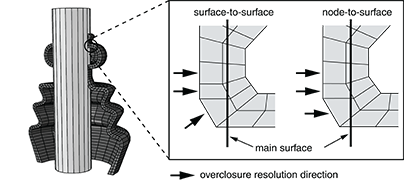
Thus, specifying a positive value for $v (t)$ causes Abaqus/Standard to ignore penetrations up to that magnitude. Figure 1 illustrates a typical interference fit problem.

If the penetration in the model is $h$ , you may declare $v = h$ or request an automatic shrink fit. In either case Abaqus/Standard will consider the two bodies to be just in contact at the start of the simulation. As the allowable interference, $v$ , is decreased during the step, Abaqus/Standard pushes the surfaces apart until there is no more allowable penetration.

There are three different ways in which to specify the allowable interference, $v$ . By default, in all cases the value of the specified allowable interference is applied instantaneously at the start of the step and then ramped down to zero linearly over the step, unless you specify an amplitude reference that defines a particular allowable interference-time variation. It is recommended that you specify allowable interferences in a step separate from the rest of the analysis; additional loads may adversely affect the resolution of the interference fit and the response to loading with partially-resolved interferences may be non-physical. Once the overclosures are resolved, you can continue the analysis in a new step.

When the contact interference is specified, output variable COPEN does not reflect the actual overclosure value during the step; it reflects the actual value only at the end of the step.

You must specify the contact pairs or contact elements at which the allowable interference should apply.

Using a Nondefault Amplitude Curve for the Allowable Interference

You can define a time-varying allowable contact interference by creating an amplitude curve (see Amplitude Curves for details) and then referring to this curve from the contact interference definition. The amplitude will be ignored, however, if the Riks method (see Unstable Collapse and Postbuckling Analysis) is used.

Removing or Modifying the Allowable Contact Interferences

By default, only the allowable contact interferences defined or redefined by a particular contact interference definition will be modified. Alternatively, you can specify that all previously defined allowable contact interferences should be removed from the model and only those defined with this definition will remain.

Specifying the Same Allowable Contact Interference for an Entire Surface

A single allowable interference $v$ can be specified for every node on the secondary surface or every secondary node in the specified set of contact elements. The concepts of secondary nodes for the various families of contact elements are discussed in their respective sections. The specified allowable contact interferences are included in the current penetrations of the secondary nodes reported in the message file when you request detailed contact printout. Thus, any secondary node that penetrates the main surface by less than the allowable interference will be reported as being open.

Using the Automatic “Shrink” Fit Method

This method is applicable only during the first step of an analysis and requires no interference value. With this method Abaqus/Standard assigns a different $v$ to each secondary node that is equal to that node's initial penetration (or zero if the point is initially open) except for the finite-sliding, surface-to-surface formulation, in which case the same value of $v$ , corresponding to the maximum penetration of the contact pair, is assigned to all constraints that are initially closed. These automatically calculated allowable contact interferences are not included in the current penetrations reported in the message file when detailed contact printout is requested.

When the automatic “shrink” fit method is used, only the default amplitude curve, a linear ramp to zero magnitude, can be used.

Applying an Allowable Contact Interference with a Shift Vector

In this method you specify a uniform allowable interference $v$ and a direction $n$ . The allowable interference value, $v$ , defines the magnitude of a shift vector. A relative shift $v n$ is applied to the secondary nodes before Abaqus/Standard determines the contact conditions. In certain applications, such as contact simulations of threaded connectors, shifting the surfaces in a specified direction is more effective than simply allowing an interference.

Figure 2 illustrates the potential difference that can result when using an allowable contact interference with a shift vector rather than using a uniform allowable contact interference. In case (a) a shift direction $n$ is defined as well as an allowable interference $v$ , while in case (b) the standard approach is used, with an allowable interference $v$ .

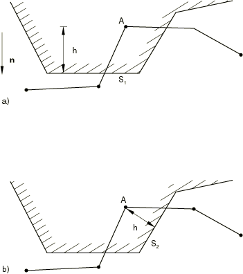
The magnitude of $v$ is the same in both cases, but it is less than the penetration in case (a) and more than the penetration in case (b). In case (a) contact is detected immediately for secondary node A, and the penetration is resolved with that node sliding along segment $s_{1}$ because node A is shifted in the direction $n$ before Abaqus/Standard checks for contact. After the shift Abaqus/Standard determines that node A is closest to segment $s_{1}$ and moves the node onto that segment. In case (b) secondary node A detects contact with segment $s_{2}$ because that is the closest segment when node A remains in its initial position. Thus, node A will slide along segment $s_{2}$ if no shift direction is provided.

Interference Fits for Surface-to-Surface Discretization

Because contact conditions are enforced in an average sense in a region around each constraint location for surface-to-surface contact, penetrations or gaps may be observed at secondary nodes when surface-to-surface constraints are in a zero-penetration state.

Large interferences may be difficult to resolve with the finite-sliding, surface-to-surface formulation. Using this formulation, overclosures tend to be resolved along the secondary facet normal directions; using node-to-surface contact, overclosures tend to be resolved along the main surface normal directions. Figure 3 illustrates a case where differing normal directions lead to undesirable tangential motion during an interference fit. In some cases it may be preferable to resolve large initial overclosures with node-to-surface discretization.

Friction and Contact Interferences

Frequently, an actual assembly process is modeled as an interference fit problem. If frictional interface properties are desired, they should usually be introduced after the initial interference has been resolved. The initial interference problem should be modeled under frictionless conditions since the physical assembly process is not typically modeled exactly. Friction can be introduced in subsequent steps (see Changing Friction Properties during an Abaqus/Standard Analysis).