Plasticity Corrections

Many types of engineering applications require the solution of nonlinear elastic-plastic problems. The finite element analysis method provides a robust way of obtaining such results accurately. However, performing a nonlinear, elastic-plastic analysis can be computationally expensive.

The Neuber and Glinka plasticity correction rules available in Abaqus/Standard provide an effective method to approximate the elastic-plastic stress and strain solution by performing only a linear elastic analysis, which can significantly reduce the computational cost. This is particularly important in concept design optimization workflows, where the analysis must be performed multiple times. The plasticity correction capabilities are also supported in static linear perturbation steps with multiple load cases, which can further substantially decrease the computational cost of the analysis.

The plasticity corrections provide postprocessed output results based on the evaluation of the Neuber or Glinka rules applied to a linear elastic response, but they do not affect the linear solution. Their evaluation is triggered by an output request, as described in Output.

Although the output variables associated with the Neuber and Glinka corrections are available only when the material response is purely elastic, their evaluation still requires knowledge of the plastic properties of the material. The plastic properties are used only to evaluate the additional plasticity corrections output variables; other solution results, which are based on linear elasticity, are not affected. You can define the plastic response for the evaluation of plasticity corrections by specifying:

• the coefficients of the Ramberg-Osgood model,
• the tabular definition of the hardening curve, or
• an elastic-plastic material definition with isotropic von Mises plasticity.

In the latter case, the plasticity corrections are evaluated only in static perturbation procedures, where the material response is always assumed to be purely elastic.

PLASTICITY CORRECTION, DEFINITION=RAMBERG-OSGOOD

PLASTICITY CORRECTION, DEFINITION=TABULAR

Neuber’s rule is one of the most widely used methods for estimating the elastic-plastic stress and strain response from purely elastic stress results. It assumes that the stress-strain product of the elastic solution is equal to the stress-strain product of the elastic-plastic solution. It can be expressed as

This is depicted graphically in Figure 1 and means that the areas of the two triangles shown in the picture must be equal. The dashed line is called the Neuber hyperbola, and the solution to the problem lies on this line. To obtain Neuber's stress and strain, ${\sigma }^N$ and ${\epsilon }^N$ , Abaqus solves the above equation together with the relationship describing the plastic response.

Figure 1. Graphical depiction of Neuber's rule.

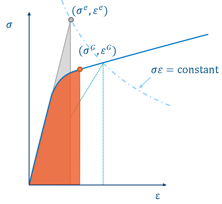
Glinka’s rule, also known as the equivalent strain energy density method (ESED), is based on the assumption that the strain energy density distribution in the localized plastic region near a notch is the same as that predicted from a linear elastic solution. This approach generally leads to smaller values of stress and strain compared to the Neuber’s rule. The corrected stress-strain response corresponds to a point on the elastic-plastic curve such that the area under the curve is equal to the area of the triangle under the purely elastic response, as shown in Figure 2. The figure also shows the triangle representing the Neuber response for comparison. Glinka's rule can be expressed as

Similarly, as in the case of Neuber's method, to obtain Glinka's stress and strain, ${\sigma }^G$ and ${\epsilon }^G$ , Abaqus solves the above equation together with the relationship describing the plastic response.

Figure 2. Graphical depiction of Glinka's rule.

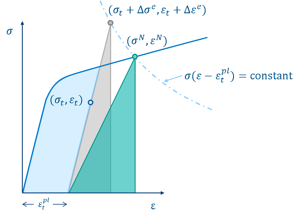
When the static perturbation step follows a general step, the elastic stress, ${\sigma }^e$ , that is used to evaluate the plasticity corrections is taken as the sum of the base stress and the perturbation stress. In addition, if plasticity corrections are requested for elements that have an elastic-plastic material definition, the corrections are evaluated taking into account the fully nonlinear elastic-plastic state of the material at the end of the general step. In this case, the modified Neuber and Glinka rules, graphically depicted in Figure 3 and Figure 4, are used to compute the corrected stresses and strains. The base value of the equivalent plastic strain is taken into account when the yield stress is evaluated, and the strain is shifted to account for the change of the stress-free configuration.

Figure 3. Graphical depiction of the modified Neuber's rule.

Figure 4. Graphical depiction of the modified Glinka's rule.

References

Molski, K., and G. Glinka, “A Method of Elastic-Plastic Stress and Strain Calculation at a Notch Root,” Materials Science and Engineering, vol. 50, pp. 93–100, 1981.
Neuber, H., “Theory of Stress Concentration for Shear-Strained Prismatical Bodies with Arbitrary Nonlinear Stress-Strain Law,” Journal of Applied Mechanics, vol. 28, pp. 544–550, 1961.