Critical State (Clay) Plasticity Model

The clay plasticity model provided in Abaqus:

describes the inelastic behavior of the material by a yield function that depends on the three stress invariants, an associated flow assumption to define the plastic strain rate, and a strain hardening theory that changes the size of the yield surface according to the inelastic volumetric strain;
can have an isotropic or an anisotropic yield function;
requires that the elastic part of the deformation be defined by using the isotropic or orthotropic linear elastic material model (Linear Elastic Behavior) or, in Abaqus/Standard, the porous elastic material model (Elastic Behavior of Porous Materials) within the same material definition (porous elasticity is supported only for isotropic yield functions);
allows for the hardening law to be defined by a piecewise linear form or, in Abaqus/Standard, by an exponential form;
may optionally include hardening in hydrostatic tension; and
can be used in conjunction with a regularization scheme for mitigating mesh dependence in situations where the material exhibits strain localization with increasing plastic deformation.

This page discusses:

Yield Surface
Hardening Law
Softening Regularization
Calibration
Initial Conditions
Elements
Output

Yield Surface

The model is based on the yield surface

\frac{1}{β^{2}} {(\frac{p - p_{t}}{a} - 1)}^{2} + {(\frac{\tilde{t}}{M a})}^{2} - 1 = 0,

where

$p = - \frac{1}{3} trace σ$: is the equivalent pressure stress;
$\tilde{t} = \frac{1}{2} \tilde{q} [1 + \frac{1}{K} - (1 - \frac{1}{K}) \cos 3 Θ]$: is the deviatoric stress measure;
$Θ$: is the deviatoric polar angle defined as $\cos 3 Θ = {(\frac{r}{q})}^{3}$ ;
$\tilde{q}$: is the Hill's potential, as defined in Hill Anisotropic Yield/Creep;
$q = \sqrt{\frac{3}{2} S : S}$: is the Mises equivalent stress;
$r = {(\frac{9}{2} S : S \cdot S)}^{\frac{1}{3}}$: is the third stress invariant;
M: is a constant that defines the slope of the critical state line;
$β$: is a constant that is equal to 1.0 on the “dry” side of the critical state line ( $p < a + p_{t}$ ) but may be different from 1.0 on the “wet” side of the critical state line ( $β \neq 1.0$ introduces a different ellipse on the wet side of the critical state line; i.e., a tighter “cap” is obtained if $β < 1.0$ as shown in Figure 1);
$a = \frac{p_{c} - p_{t}}{(1 + β)}$: is a measure of the size of the yield surface (Figure 1);
$p_{c}$: is the yield stress in hydrostatic compression;
$p_{t}$: is the yield stress in hydrostatic tension; and
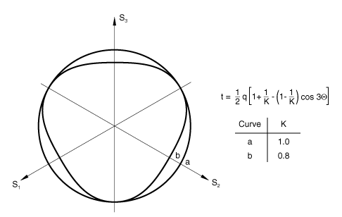
K: is the ratio of the flow stress in triaxial tension to the flow stress in triaxial compression and determines the shape of the yield surface in the plane of principal deviatoric stresses (the “ $Π$ -plane”: see Figure 2); Abaqus requires that $0.778 \leq K \leq 1.0$ to ensure that the yield surface remains convex.

The user-defined parameters M, $β$ , and K can depend on temperature $θ$ as well as other predefined field variables, $f_{i}$ . For the isotropic model, the expression for $\tilde{q}$ reduces to the Mises equivalent stress, $q$ . The model is described in detail in Critical state models.

Hardening Law

The hardening law can have an exponential form (Abaqus/Standard only) or a piecewise linear form.

Exponential Form in Abaqus/Standard

The exponential form of the hardening law can be used only in conjunction with the Abaqus/Standard porous elastic material model and the isotropic form of the yield surface with $p_{t} = 0$ . The size of the yield surface at any time is determined by the initial value of the hardening parameter, $a_{0}$ , and the amount of inelastic volume change that occurs according to the equation

a = a_{0} \exp [(1 + e_{0}) \frac{1 - J^{p l}}{λ - κ J^{p l}}],

where

$J^{p l}$: is the inelastic volume change (that part of J, the ratio of current volume to initial volume, attributable to inelastic deformation);
$κ (θ, f_{i})$: is the logarithmic bulk modulus of the material defined for the porous elastic material behavior;
$λ (θ, f_{i})$: is the logarithmic hardening constant defined for the clay plasticity material behavior; and
$e_{0}$: is the user-defined initial void ratio (Defining Initial Void Ratios in a Porous Medium).

Specifying the Initial Size of the Yield Surface Directly

The initial size of the yield surface is defined for clay plasticity by specifying the hardening parameter, $a_{0}$ , as a tabular function or by defining it analytically.

$a_{0}$ can be defined along with $λ$ , M, $β$ , and K, as a tabular function of temperature and other predefined field variables. However, $a_{0}$ is a function only of the initial conditions; it will not change if temperatures and field variables change during the analysis.

Specifying the Initial Size of the Yield Surface Indirectly

The hardening parameter $a_{0}$ can be defined indirectly by specifying $e_{1}$ , which is the intercept of the virgin consolidation line with the void ratio axis in the plot of void ratio, e, versus the logarithm of the effective pressure stress, $\ln p$ (Figure 3).

If this method is used, $a_{0}$ is defined by

a_{0} = \frac{1}{2} \exp (\frac{e_{1} - e_{0} - κ \ln p_{0}}{λ - κ}),

where $p_{0}$ is the user-defined initial value of the equivalent hydrostatic pressure stress (see Defining Initial Stresses). You define $e_{1}$ , $λ$ , M, $β$ , and K; all the parameters except $e_{1}$ can be dependent on temperature and other predefined field variables. However, $a_{0}$ is a function only of the initial conditions; it will not change if temperatures and field variables change during the analysis.

Piecewise Linear Form

If the piecewise linear form of the hardening rule is used, the user-defined relationship relates the yield stress in hydrostatic compression, $p_{c}$ , and, optionally, the yield stress in hydrostatic tension, $p_{t}$ , to the corresponding volumetric plastic strain, $ε_{vol}^{p l}$ (Figure 4):

p_{c} = p_{c} (ε_{vol}^{p l}),

p_{t} = p_{t} (ε_{vol}^{p l}) .

The evolution parameter, a, is then given by

a = \frac{p_{c} - p_{t}}{(1 + β)} .

The volumetric plastic strain axis has an arbitrary origin: ${ε_{vol}^{p l} |}_{0}$ is the position on this axis corresponding to the initial state of the material, thus defining the initial hydrostatic pressure in compression, ${p_{c} |}_{0}$ , and, optionally, in tension, ${p_{t} |}_{0}$ and, hence, the initial yield surface size, $a_{0}$ . This relationship is defined in tabular form as clay hardening data. The range of values for which $p_{c}$ and $p_{t}$ is defined should be sufficient to include all values of equivalent pressure stress to which the material will be subjected during the analysis. Data for $p_{c}$ must be specified; data for $p_{t}$ is optional.

This form of the hardening law can be used in conjunction with either the linear elastic or, in Abaqus/Standard, the porous elastic material models. This is the only form of the hardening law supported in Abaqus/Explicit.

Softening Regularization

Granular materials often exhibit strain localization with increasing plastic deformation. Post-failure solutions from conventional finite element methods can be strongly mesh dependent. To mitigate the mesh dependency of the solutions, a regularization method is often used to introduce a micro-structural length scale into the constitutive formulation. Let $l_{c}^{(m)}$ denote the characteristic width of a shear band or a crack band, $l_{c}^{(e)}$ the characteristic length of the element, and $ε_{vol, e}^{p l}$ the inelastic strain for the element. Then the inelastic strain in the localization band, $ε_{vol, m}^{p l}$ , is defined to be

ε_{vol, m}^{p l} = ε_{vol, e}^{p l} min ({(\frac{l_{c}^{(e)}}{l_{c}^{(m)}})}^{n_{r}}, f_{m a x}),

where $n_{r}$ is a material parameter and $f_{m a x}$ is a positive number used for bounding the magnitude of regularization. This strain regularization method is valid only when the characteristic length of the element is greater than the width of the localization band; i.e., $l_{c}^{(e)} \geq l_{c}^{(m)}$ .

If softening regularization is included, it is applied to all hardening data (tension and compression) by default. You can optionally turn off softening regularization for a specific type of hardening.

Calibration

At least two experiments are required to calibrate the simplest version of the Cam-clay model: a hydrostatic compression test (an oedometer test is also acceptable) and a triaxial compression test (more than one triaxial test is useful for a more accurate calibration).

Hydrostatic Compression Tests

The hydrostatic compression test is performed by pressurizing the sample equally in all directions. The applied pressure and the volume change are recorded.

The onset of yielding in the hydrostatic compression test immediately provides the initial position of the yield surface, $a_{0}$ . The logarithmic bulk moduli, $κ$ and $λ$ , are determined from the hydrostatic compression experimental data by plotting the logarithm of pressure versus void ratio. The void ratio, e, is related to the measured volume change as

J = \exp (ε_{v o l}) = \frac{1 + e}{1 + e_{0}} .

The slope of the line obtained for the elastic regime is $- κ$ , and the slope in the inelastic range is $- λ$ . For a valid model $λ > κ$ .

Triaxial Tests

Triaxial compression experiments are performed using a standard triaxial machine where a fixed confining pressure is maintained while the differential stress is applied. Several tests covering the range of confining pressures of interest are usually performed. Again, the stress and strain in the direction of loading are recorded, together with the lateral strain so that the correct volume changes can be calibrated.

The triaxial compression tests allow the calibration of the yield parameters M and $β$ . M is the ratio of the shear stress, q, to the pressure stress, p, at critical state and can be obtained from the stress values when the material has become perfectly plastic (critical state). $β$ represents the curvature of the cap part of the yield surface and can be calibrated from a number of triaxial tests at high confining pressures (on the “wet” side of critical state). $β$ must be between 0.0 and 1.0.

To calibrate the parameter K, which controls the yield dependence on the third stress invariant, experimental results obtained from a true triaxial (cubical) test are necessary. These results are generally not available, and you may have to guess (the value of K is generally between 0.8 and 1.0) or ignore this effect.

To calculate the yield stress in hydrostatic tension, you can plot the data obtained from the triaxial compression tests on the $p$ – $q$ plane and extend the curve obtained from fitting these experimental data to the pressure axis in the tensile region.

Unloading Measurements

Unloading measurements in hydrostatic and triaxial compression tests are useful to calibrate the elasticity, particularly in cases where the initial elastic region is not well defined. From these we can identify whether a constant shear modulus or a constant Poisson's ratio should be used and what their values are.

Initial Conditions

If an initial stress at a point is given (see Defining Initial Stresses) such that the stress point lies outside the initially defined yield surface, Abaqus will try to adjust the initial position of the surface to make the stress point lie on it and issue a warning. However, if the yield stress in hydrostatic tension, $p_{t}$ , is zero and does not evolve with volumetric plastic strain and the stress point is such that the equivalent pressure stress, p, is negative, an error message will be issued and execution will be terminated.

The initial condition on volumetric plastic strain, ${ε_{vol}^{p l} |}_{0}$ , can be defined in the definition of the clay plasticity model. Abaqus also allows a general method of specifying the initial plastic strain field on elements (see Defining Initial Values of Plastic Strain). The volumetric plastic strain is then calculated as

ε_{vol}^{p l} = {ε_{vol}^{p l} |}_{0} - t r (ε^{p l}) .

Elements

The clay plasticity model can be used with plane strain, generalized plane strain, axisymmetric, and three-dimensional solid (continuum) elements in Abaqus. This model cannot be used with elements for which the assumed stress state is plane stress (plane stress, shell, and membrane elements).

Output

In addition to the standard output identifiers available in Abaqus (Abaqus/Standard Output Variable Identifiers and Abaqus/Explicit Output Variable Identifiers), the following variable has special meaning for material points in the clay plasticity model:

PEEQ: Center of the yield surface, a.