Thermal Expansion

Thermal expansion effects:

can be defined by specifying thermal expansion coefficients so that Abaqus can compute thermal strains;
can be isotropic, orthotropic, or fully anisotropic;
are defined as total expansion from a reference temperature;
can be specified as a function of temperature and/or field variables;
can be defined with a distribution for solid continuum elements in Abaqus/Standard; and
can be specified directly in Abaqus/Standard in user subroutine UEXPAN or in Abaqus/Explicit in user subroutine VUEXPAN if the thermal strains are complicated functions of temperature, time, field variables, and state variables.

This page discusses:

Defining Thermal Expansion Coefficients
Computing Thermal Strains in Linear Perturbation Steps
Defining Increments of Thermal Strain in User Subroutines
Defining the Initial Temperature and Field Variable Values
Defining Directionally Dependent Thermal Expansion
Defining Thermal Expansion for a Short-Fiber Reinforced Composite
Thermal Stress
Material Options
Elements
References

Defining Thermal Expansion Coefficients

Thermal expansion is a material property included in a material definition (see Material Data Definition) except when it refers to the expansion of a gasket whose material properties are not defined as part of a material definition. In that case expansion must be used in conjunction with the gasket behavior definition (see Defining the Gasket Behavior Directly Using a Gasket Behavior Model).

In an Abaqus/Standard analysis a spatially varying thermal expansion can be defined for homogeneous solid continuum elements by using a distribution (Distribution Definition). The distribution must include default values for the thermal expansion. If a distribution is used, no dependencies on temperature and/or field variables for the thermal expansion can be defined.

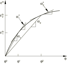
Computation of Thermal Strains

Abaqus requires thermal expansion coefficients, $α$ , that define the total thermal expansion from a reference temperature, $θ^{0}$ , as shown in Figure 1.

They generate thermal strains according to the formula

ε^{t h} = α (θ, f_{β}) (θ - θ^{0}) - α (θ^{I}, f_{β}^{I}) (θ^{I} - θ^{0}),

where

$α (θ, f_{β})$: is the thermal expansion coefficient;
$θ$: is the current temperature;
$θ^{I}$: is the initial temperature;
$f_{β}$: are the current values of the predefined field variables;
$f_{β}^{I}$: are the initial values of the field variables; and
$θ^{0}$: is the reference temperature for the thermal expansion coefficient.

The second term in the above equation represents the strain due to the difference between the initial temperature, $θ^{I}$ , and the reference temperature, $θ^{0}$ . This term is necessary to enforce the assumption that there is no initial thermal strain for cases in which the reference temperature does not equal the initial temperature.

Defining the Reference Temperature

If the coefficient of thermal expansion, $α$ , is not a function of temperature or field variables, the value of the reference temperature, $θ^{0}$ , is not needed. If $α$ is a function of temperature or field variables, you can define $θ^{0}$ .

Converting Thermal Expansion Coefficients from Differential Form to Total Form

Total thermal expansion coefficients are commonly available in tables of material properties. However, sometimes you are given thermal expansion data in differential form:

d ε^{t h} = α^{'} (θ) d θ;

that is, the tangent to the strain-temperature curve is provided (see Figure 1). To convert to the total thermal expansion form required by Abaqus, this relationship must be integrated from a suitably chosen reference temperature, $θ^{0}$ :

ε^{t h} = \int_{θ^{0}}^{θ} α^{'} d θ \Rightarrow α (θ) = \frac{1}{θ - θ^{0}} \int_{θ^{0}}^{θ} α^{'} d θ .

For example, suppose $α^{'}$ is a series of constant values: $α_{1}^{'}$ between $θ^{0}$ and $θ^{1}$ ; $α_{2}^{'}$ between $θ^{1}$ and $θ^{2}$ ; $α_{3}^{'}$ between $θ^{2}$ and $θ^{3}$ ; etc. Then,

\begin{matrix} ε_{1}^{t h} = & α_{1}^{'} (θ^{1} - θ^{0}) \\ ε_{2}^{t h} = & ε_{1}^{t h} + α_{2}^{'} (θ^{2} - θ^{1}) \\ ε_{3}^{t h} = & ε_{2}^{t h} + α_{3}^{'} (θ^{3} - θ^{2}) . \end{matrix}

The corresponding total expansion coefficients required by Abaqus are then obtained as

\begin{matrix} α_{1} = & ε_{1}^{t h} / (θ^{1} - θ^{0}) \\ α_{2} = & ε_{2}^{t h} / (θ^{2} - θ^{0}) \\ α_{3} = & ε_{3}^{t h} / (θ^{3} - θ^{0}) . \end{matrix}

Computing Thermal Strains in Linear Perturbation Steps

During a linear perturbation step, temperature perturbations can produce perturbations of thermal strains in the form:

Δ ε^{t h} = α^{'} (θ^{B}) Δ θ,

where $Δ θ$ is the temperature perturbation load about the base state, $θ^{B}$ is the temperature in the base state, and $α^{'} (θ^{B})$ is the tangent thermal expansion coefficient evaluated in the base state. Abaqus computes the tangent thermal expansion coefficients from the total form as

α^{'} (θ) = \frac{\partial ε^{t h}}{\partial θ} = α + \frac{\partial α}{\partial θ} (θ - θ^{0}) .

Defining Increments of Thermal Strain in User Subroutines

Increments of thermal strain can be specified in user subroutine UEXPAN in Abaqus/Standard and in user subroutine VUEXPAN in Abaqus/Explicit as functions of temperature and/or predefined field variables. User subroutine UEXPAN in Abaqus/Standard must be used if the thermal strain increments depend on state variables.

Defining the Initial Temperature and Field Variable Values

If the coefficient of thermal expansion, $α$ , is a function of temperature or field variables, the initial temperature and initial field variable values, $θ^{I}$ and $f_{β}^{I}$ , are given as described in Initial Conditions.

Element Removal and Reactivation

If an element has been removed and subsequently reactivated in Abaqus/Standard (Element and Contact Pair Removal and Reactivation), $θ^{I}$ and $f_{β}^{I}$ in the equation for the thermal strains represent temperature and field variable values as they were at the moment of reactivation.

Defining Directionally Dependent Thermal Expansion

Isotropic, orthotropic, and fully anisotropic thermal expansion can be defined in Abaqus.

Orthotropic and anisotropic thermal expansion can be used only with materials where the material directions are defined with local orientations (see Orientations).

Isotropic Expansion

If the thermal expansion coefficient is defined directly, only one value of $α$ is needed at each temperature. If user subroutine UEXPAN is used, only one isotropic thermal strain increment ( $Δ ε = Δ ε_{11} = Δ ε_{22} = Δ ε_{33}$ ) must be defined.

Orthotropic Expansion

If the thermal expansion coefficients are defined directly, the three expansion coefficients in the principal material directions ( $α_{11}$ , $α_{22}$ , and $α_{33}$ ) should be given as functions of temperature. If user subroutines UEXPAN and VUEXPAN are used, the three components of thermal strain increment in the principal material directions ( $Δ ε_{11}$ , $Δ ε_{22}$ , and $Δ ε_{33}$ ) must be defined.

Anisotropic Expansion

If the thermal expansion coefficients are defined directly, all six components of $α$ ( $α_{11}$ , $α_{22}$ , $α_{33}$ , $α_{12}$ , $α_{13}$ , $α_{23}$ ) must be given as functions of temperature. If user subroutine UEXPAN is used in Abaqus/Standard, all six components of the thermal strain increment ( $Δ ε_{11}$ , $Δ ε_{22}$ , $Δ ε_{33}$ , $Δ ε_{12}$ , $Δ ε_{13}$ , $Δ ε_{23}$ ) must be defined. If user subroutine VUEXPAN is used in Abaqus/Explicit, all six components of the thermal strain increment ( $Δ ε_{11}$ , $Δ ε_{22}$ , $Δ ε_{33}$ , $Δ ε_{12}$ , $Δ ε_{23}$ , $Δ ε_{13}$ ) must be defined.

In an Abaqus/Standard analysis if a distribution is used to define the thermal expansion, the number of expansion coefficients given for each element in the distribution, which is determined by the associated distribution table (Distribution Definition), must be consistent with the level of anisotropy specified for the expansion behavior. For example, if orthotropic behavior is specified, three expansion coefficients must be defined for each element in the distribution.

Defining Thermal Expansion for a Short-Fiber Reinforced Composite

The thermal expansion coefficient of a short-fiber reinforced composite (for example, an injection molded composite) can be computed using the orientation averaging described by Zheng (2011):

〈 α 〉 = {〈 D^{U D} 〉}^{- 1} 〈 D^{U D} α^{U D} 〉,

where $〈 D^{U D} 〉$ is the orientation-averaged elasticity matrix computed using the elasticity of the unidirectional (UD) composite and the second-order orientation tensor (see Defining the Elasticity of a Short-Fiber Reinforced Composite), and $〈 D^{U D} α^{U D} 〉$ is given by:

〈 D_{i j k l}^{U D} α_{k l}^{U D} 〉 = [(D_{1111}^{U D} - D_{1122}^{U D}) α_{11}^{U D} + (2 D_{1122}^{U D} - D_{2222}^{U D} - D_{2233}^{U D}) α_{22}^{U D}] a_{i j} + [D_{2211}^{U D} α_{11}^{U D} + (D_{2222}^{U D} + D_{2233}^{U D}) α_{22}^{U D}] δ_{i j},

where $D^{U D}$ and $α^{U D}$ are the elasticity matrix and thermal expansion coefficient of the unidirectional composite with the 1-direction as the fiber direction, $a_{i j}$ is the second-order orientation tensor, and $δ_{i j}$ is the Kronecker delta. The unidirectional composite is assumed to be transversely isotropic. Similar to elasticity, you must define the material directions with local orientations (see Orientations), and the axes of the local system must align with the principal directions of the second-order orientation tensor.

Thermal Stress

When a structure is not free to expand, a change in temperature will cause stress. For example, consider a single two-node truss of length L that is completely restrained at both ends. The cross-sectional area; the Young's modulus, E; and the thermal expansion coefficient, $α$ , are all constant. The stress in this one-dimensional problem can then be calculated from Hooke's Law as $σ_{x} = E (ε_{x} - ε_{x}^{t h})$ , where $ε_{x}$ is the total strain and $ε_{x}^{t h} = α Δ θ$ is the thermal strain, where $Δ θ$ is the temperature change. Since the element is fully restrained, $ε_{x} = 0$ . If the temperature at both nodes is the same, we obtain the stress $σ_{x} = - E α Δ θ$ .

Constrained thermal expansion can cause significant stress. For typical structural metals, temperature changes of about 150°C (300°F) can cause yield. Therefore, it is often important to define boundary conditions with particular care for problems involving thermal loading to avoid overconstraining the thermal expansion.

Energy Balance Considerations

Abaqus does not account for thermal expansion effects in the total energy balance equation, which can lead to an apparent imbalance of the total energy of the model. For example, in the example above of a two-node truss restrained at both ends, constrained thermal expansion introduces strain energy that will result in an equivalent increase in the total energy of the model.

Material Options

Thermal expansion can be combined with any other (mechanical) material (see Combining Material Behaviors) behavior in Abaqus.

Using Thermal Expansion with Other Material Models

For most materials thermal expansion is defined by a single coefficient or set of orthotropic or anisotropic coefficients or, in Abaqus/Standard, by defining the incremental thermal strains in user subroutine UEXPAN. For porous media in Abaqus/Standard, such as soils or rock, thermal expansion can be defined for the solid grains and for the permeating fluid (when using the coupled pore fluid diffusion/stress procedure—see Coupled Pore Fluid Diffusion and Stress Analysis). In such a case the thermal expansion definition should be repeated to define the different thermal expansion effects.

Using Thermal Expansion with Gasket Behaviors

Thermal expansion can be used in conjunction with any gasket behavior definition. Thermal expansion will affect the expansion of the gasket in the membrane direction and/or the expansion in the gasket's thickness direction.

Elements

Thermal expansion can be used with any stress/displacement or fluid element in Abaqus.

References

Zheng, R., R. I. Tanner, and X. Fan, Injection Molding: Integration of Theory and Modeling Methods, Springer, 2011.