Conventions

The conventions that are used throughout Abaqus are defined in this section.

This page discusses:

Degrees of Freedom
Coordinate Systems
Units
Time Measures
Local Tangent Directions on Surfaces in Space
Convention Used for Stress and Strain Components
Stress and Strain Measures
Stress Invariants
Finite Rotations

Degrees of Freedom

Except for axisymmetric elements and electromagnetic elements, the degrees of freedom are always referred to as follows:


1	x-displacement
2	y-displacement
3	z-displacement
4	Rotation about the x-axis, in radians
5	Rotation about the y-axis, in radians
6	Rotation about the z-axis, in radians
7	Warping amplitude (for open-section beam elements)
8	Pore pressure, hydrostatic fluid pressure, or acoustic pressure
9	Electric potential
10	Connector material flow (units of length)
11	Temperature (or normalized concentration in mass diffusion analysis)
12	Second temperature (for shells or beams)
13	Third temperature (for shells or beams)
14	Etc.
30	20th temperature (for shells or beams)
32	Electric potential in the electrolyte
33	Ion concentration in the electrolyte

Here the x-, y-, and z-directions coincide with the global X-, Y-, and Z-directions, respectively; however, if a local transformation is defined at a node (see Transformed Coordinate Systems), they coincide with the local directions defined by the transformation.

A maximum of 20 temperature values (degrees of freedom 11 through 30) can be defined for shell or beam elements in Abaqus/Standard.

Axisymmetric Elements

The displacement and rotation degrees of freedom in axisymmetric elements are referred to as follows:


1	r-displacement
2	z-displacement
5	Rotation about the z-axis (for axisymmetric elements with twist), in radians
6	Rotation in the r–z plane (for axisymmetric shells), in radians

Here the r- and z-directions coincide with the global X- and Y-directions, respectively; however, if a local transformation is defined at a node (see Transformed Coordinate Systems), they coincide with the local directions defined by the transformation.

Electromagnetic Elements

Electromagnetic elements in Abaqus/Standard are used to define the element shape and to discretize the continuum. The eddy current and magnetostatic analyses formulations use magnetic vector potential as a degree of freedom (see Boundary Conditions and Boundary Conditions).

Activation of Degrees of Freedom

Abaqus/Standard and Abaqus/Explicit activate only those degrees of freedom needed at a node. Therefore, some of the degrees of freedom listed above may not be used at all nodes in a model, because each element type uses only those degrees of freedom that are relevant. For example, two-dimensional solid (continuum) stress/displacement elements use only degrees of freedom 1 and 2. The degrees of freedom actually used at any node are the envelope of those needed in each element that shares the node.

Internal Variables in Abaqus/Standard

In addition to the degrees of freedom listed above, Abaqus/Standard uses internal variables (such as Lagrange multipliers to impose constraints) for some elements. Normally you need not be concerned with these variables, but they may appear in error and warning messages and are checked for satisfaction of nonlinear constraints during iteration. Internal variables are always associated with internal nodes, which have negative numbers to distinguish them from user-defined nodes.

Coordinate Systems

The basic coordinate system in Abaqus is a right-handed, rectangular Cartesian system. You can choose other systems locally for input (see Node Definition), for output of nodal variables (displacements, velocities, etc.) and point load or boundary condition specification (see Transformed Coordinate Systems), and for material or kinematic joint specification (see Orientations). All coordinate systems must be right-handed.

Units

Abaqus has no units built into it except for rotation and angle measures. Therefore, the units chosen must be self-consistent, which means that derived units of the chosen system can be expressed in terms of the fundamental units without conversion factors.

Rotation and Angle Measures

In Abaqus rotational degrees of freedom are expressed in radians, and all other angle measures are expressed in degrees (for example, phase angles).

International System of Units (SI)

The International System of units (SI) is an example of a self-consistent set of units. The fundamental units in the SI system are length in meters (m), mass in kilograms (kg), time in seconds (s), temperature in degrees kelvin (K), and electric current in amperes (A). The units of secondary or derived quantities are based on these fundamental units. An example of a derived unit is the unit of force. A unit of force in the SI system is called a newton (N):

1 newton = 1 kg
  m / s^{2} .

Similarly, a unit of electrical charge in the SI system is called a coulomb (C):

1 coulomb = 1 A
  s .

Another example is the unit of energy, called a joule (J):

1 joule = 1 N
  m = 1 A volt
  s = 1 {kg
  m}^{2} / s^{2} .

The unit of electrical potential in the SI system is the volt, which is chosen such that

1 joule = 1 volt
  C = 1 volt A
  s .

Sometimes the standard units are not convenient to work with. For example, Young's modulus is frequently specified in terms of megapascals (MPa) (or, equivalently, N/mm²), where 1 pascal = 1 N/m². In this case the fundamental units could be tonnes (1 tonne = 1000 kilograms), millimeters, and seconds.

American or English Units

American or English units can cause confusion since the naming conventions are not as clear as in the SI system. For example, 1 pound force (lbf) gives 1 pound mass (lbm) an acceleration of g ft/sec², where g is the value of acceleration due to gravity. If pounds force, feet (ft), and seconds are taken as fundamental units, the derived unit of mass is lbf sec²/ft. Since density is commonly given in handbooks as lbm/in³, it must be converted to lbf sec²/ft⁴ by

1 lbm / {in}^{3} = \frac{12^{3}}{g} lbf {sec}^{2} / {ft}^{4} .

Frequently it is not made clear in handbooks whether $lb$ stands for lbm or lbf. You need to check that the values used make up a consistent set of units.

Two other units that cause difficulty are the slug, defined as the mass that is accelerated at 1 ft/sec² by 1 lbf, and the poundal, defined as the force required to accelerate 1 lbm at 1 ft/sec². Useful conversions are

1 slug = g lbm

and

1 lbf = g poundals,

where g is the magnitude of the acceleration due to gravity in ft/sec².

Symbols Used in Abaqus for Units

Units are indicated for the value to be given on load and flux types as follows:


Dimension	Indicator	Example (S.I. units)
length	L	meter
mass	M	kilogram
time	T	second
temperature	$θ$	degree Celsius
electric current	A	ampere
force	F	newton
energy	J	joule
electric charge	C	coulomb
electric potential	$φ$	volt
mass concentration	P	Parts per million
fluid electric potential	$φ_{e}$	volt
ion concentration in the electrolyte	$C_{e}$	mol per cubic meter

Defining a Unit System for an Abaqus/Standard Substructure for a Simpack Flexible Body

In Abaqus/Standard you can specify a unit system in the model to use when translating to other formats. In a matrix generation procedure, the unit system is stored on the binary SIM file containing the generated matrices. In a substructure generation procedure, the unit system is stored on the binary SIM file containing the substructure.

If you generate flexible body entities from an Abaqus/Standard substructure for the Simpack flexible body dynamics solver, you must specify units. Two approaches are available. In the first approach you specify a unit system in the Abaqus/Standard model directly. The specified unit system is not used during the substructure generation procedure. However, the unit information is stored with the substructure and is accessed during the creation of the flexible body. In the second approach (in which you do not specify the unit system), you must run the abaqus tosimpack translator in stand-alone mode and define the model units on the command line (see Translating an Abaqus Substructure to a Simpack Flexible Body).

You define the units of a mechanical system by specifying one of the basic triples: length-mass-time or length-force-time. These two methods are mutually exclusive. If you specify length-mass-time, the force unit is defined implicitly. If you specify length-force-time, the mass unit is defined implicitly. You specify a unit symbol that defines the primary conversion factor, as shown in the tables below. The primary conversion factor is the number that Abaqus multiplies by the SI unit to obtain the current model unit. For example, if the Abaqus model length unit is mm, the primary conversion factor is 0.001. To use units that are not in the list of unit symbols (such as the angstrom unit), you can specify a secondary conversion factor. This is another multiplier for the conversion from the Abaqus model units to the SI system.

Table 1. Length unit symbols.
Unit Name	Unit Symbol	Primary Conversion Factor
Meter (default)	m	1.0
Centimeter	cm	1.0E-2
Millimeter	mm	1.0E-3
Kilometer	km	1.0E+3
Inch	in	0.0254
Foot	ft	0.3048
Yard	yd	0.9144
Mile	mi	1609.344

Table 2. Mass unit symbols.
Unit Name	Unit Symbol	Primary Conversion Factor
Kilogram (default)	kg	1.0
Gram	g	1.0E-3
Tonne (metric ton)	t	1.0E+3
Pound	lb	0.45359237
Kilopound	klb	453.59237
Ounce	oz	0.0283495
Slug	slug	14.593903
Slinch (dozen slug)	slinch	175.126835246476
US ton (short ton)	uton	907.185

Table 3. Time unit symbols.
Unit Name	Unit Symbol	Primary Conversion Factor
Second (default)	s	1.0
Millisecond	ms	1.0E-3
Hour	h	3600.0
Minute	min	60.0
Day	d	86400.0

Table 4. Force unit symbols.
Unit Name	Unit Symbol	Primary Conversion Factor
Newton (default)	N	1.0
Pound-force	lbf	4.44822161526
Kilogram-force	kgf	9.80665
Ounce-force	ozf	0.2780139
Dyne	dyne	1.0E-5
Kilonewton	kN	1.0E+3
Kilopound-force	klbf	4448.22161526
Tonne-force	tf	9.80665E+3
Poundal	pdl	0.138254954

Time Measures

Abaqus has two measures of time—step time and total time. Except for certain linear perturbation procedures, step time is measured from the beginning of each step. Total time starts at zero and is the total accumulated time over all general analysis steps (including restart steps; see Restarting an Analysis). Total time does not accumulate during linear perturbation steps.

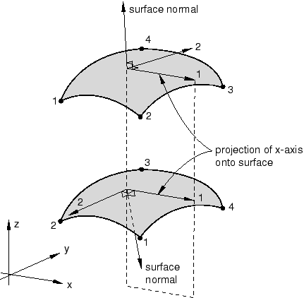
Local Tangent Directions on Surfaces in Space

Local tangent directions are needed on surfaces in space; for example, to provide a convention for describing components of slip on an element-based contact surface or components of stress and strain in a shell. The convention used in Abaqus for such directions is as follows.

The default local 1-direction is the projection of the global x-axis onto the surface. If the global x-axis is within 0.1° of being normal to the surface, the local 1-direction is the projection of the global z-axis onto the surface. The local 2-direction is then at right angles to the local 1-direction, so that the local 1-direction, local 2-direction, and the positive normal to the surface form a right-handed set (see Figure 1). The positive normal direction is defined in an element by the right-hand rotation rule going around the nodes of the element. The local surface directions can be redefined; see Orientations.

The local 1- and 2-directions become local 2- and 3-directions, respectively, when considering gasket elements or the local systems associated with integrated output sections (Integrated Output Section Definition) or user-defined sections (Section Output from Abaqus/Standard).

For “line”-type surfaces defined on beam, pipe, or truss elements in space, the default local 1-direction and 2-direction are tangential and transverse to the elements. In this case the local surface directions can also be redefined as described in Orientations.

Rotation of the Local Directions

For geometrically linear analysis, stress and strain components are given by default in the material directions in the reference (initial) configuration.

For geometrically nonlinear analysis, small-strain shell elements in Abaqus/Standard (S4R5, S8R, S8R5, S8RT, S9R5, STRI3, and STRI65) use a total Lagrangian strain, and the stress and strain components are given relative to material directions in the reference configuration. Gasket elements are small-strain small-displacement elements, and the components are output by default in the behavior directions in the reference configuration.

For finite-membrane-strain elements (all membrane elements, S3/S3R, S4, S4R, SAX, and SAXA elements) and for small-strain shell elements in Abaqus/Explicit, the material directions rotate with the average rigid body motion of the surface to form the material directions in the current configuration. Stress and strain components in these elements are given relative to these material directions in the current configuration.

For a more thorough discussion of the definition of the rotated coordinate directions in membrane elements; S3/S3R, S4, and S4R elements; S3RS, S4RS, and S4RSW elements; and SAXA elements, see:

You can determine whether the local system associated with a user-defined section is fixed or rotates with the average rigid body motion; see Section Output from Abaqus/Standard for details.

You can determine whether the local system associated with an integrated output section is fixed, translates with average rigid body motion, or translates and rotates with the average rigid body motion; see Integrated Output Section Definition for details.

See Contact Formulations in Abaqus/Standard for information on how the local tangent directions evolve during an Abaqus/Standard contact analysis.

Convention Used for Stress and Strain Components

When defining material properties, the convention used for stress and strain components in Abaqus is that they are ordered:


$σ_{11}$	Direct stress in the 1-direction
$σ_{22}$	Direct stress in the 2-direction
$σ_{33}$	Direct stress in the 3-direction
$τ_{12}$	Shear stress in the 1–2 plane
$τ_{13}$	Shear stress in the 1–3 plane
$τ_{23}$	Shear stress in the 2–3 plane

For example, a fully anisotropic, linear elasticity matrix is

(\begin{matrix} σ_{11} \\ σ_{22} \\ σ_{33} \\ τ_{12} \\ τ_{13} \\ τ_{23} \end{matrix}) = [\begin{matrix} D_{1111} & D_{1122} & D_{1133} & D_{1112} & D_{1113} & D_{1123} \\ D_{2222} & D_{2233} & D_{2212} & D_{2213} & D_{2223} \\ D_{3333} & D_{3312} & D_{3313} & D_{3323} \\ symm. & D_{1212} & D_{1213} & D_{1223} \\ D_{1313} & D_{1323} \\ D_{2323} \end{matrix}] (\begin{matrix} ε_{11} \\ ε_{22} \\ ε_{33} \\ γ_{12} \\ γ_{13} \\ γ_{23} \end{matrix}) .

The 1-, 2-, and 3-directions depend on the element type chosen. For solid elements the defaults for these directions are the global spatial directions. For shell and membrane elements the defaults for the 1- and 2-directions are local directions in the surface of the shell or membrane, as defined in About the Element Library. In both cases the 1-, 2-, and 3-directions can be changed as described in Orientations.

For geometrically nonlinear analysis with solid elements, the default (global) directions do not rotate with the material. However, user-defined orientations do rotate with the material.

Abaqus/Explicit stores the stress and strain components internally in a different order: $σ_{11}$ , $σ_{22}$ , $σ_{33}$ , $τ_{12}$ , $τ_{23}$ , $τ_{13}$ . For geometrically nonlinear analysis, the internally stored components rotate with the material, regardless of whether or not a user-defined orientation is used. This distinction is important when a user subroutine (such as VUMAT) is used.

Nonisotropic Material Behavior

When nonisotropic material behavior is defined in continuum elements, a user-defined orientation is necessary for the anisotropic behavior to be associated with material directions. See State storage for a description of how material directions rotate.

Zero-Valued Stress Components

Stress components that are always zero are omitted from storage. For example, in plane stress Abaqus stores only the two direct components and one shear component of stress and strain in the plane where the stress values are nonzero.

Shear Strains

Abaqus always reports shear strain as engineering shear strain, $γ$ :

γ_{i j} = ε_{i j} + ε_{j i} .

Stress and Strain Measures

The stress measure used in Abaqus is Cauchy or “true” stress, which corresponds to the force per current area. See Stress measures and Stress rates for more details on stress measures.

For geometrically nonlinear analysis, a large number of different strain measures exist. Unlike “true” stress, there is no clearly preferred “true” strain. For the same physical deformation different strain measures report different values in large-strain analysis. The optimal choice of strain measure depends on analysis type, material behavior, and (to some degree) personal preference. See Strain measures for more details on strain measures.

By default, the strain output in Abaqus/Standard is the “integrated” total strain (output variable E). For large-strain shells, membranes, and solid elements in Abaqus/Standard two other measures of total strain can be requested: logarithmic strain (output variable LE) and nominal strain (output variable NE).

Logarithmic strain (output variable LE) is the default strain output in Abaqus/Explicit; nominal strain (output variable NE) can be requested as well. The “integrated” total strain is not available in Abaqus/Explicit.

Total (Integrated) Strain

The default “integrated” strain measure, E, output by Abaqus/Standard to the data (.dat) and results (.fil) files for all elements that can handle finite strain is obtained by integrating the strain rate numerically in a material frame of reference:

ε^{n + 1} = Δ R \cdot ε^{n} \cdot Δ R^{T} + Δ ε,

where $ε^{n + 1}$ and $ε^{n}$ are the total strains at increments $n + 1$ and n, respectively; $Δ R$ is the incremental rotation tensor; and $Δ ε$ is the total strain increment from increment n to $n + 1$ . For elements that use a corotational coordinate system (finite-strain shells, membranes, and solid elements with user-defined orientations), the above equation simplifies to

ε^{n + 1} = ε^{n} + Δ ε .

The strain increment is obtained by integration of the rate of deformation $D$ over the time increment:

Δ ε = \int_{t^{n}}^{t^{n + 1}} D d t .

This strain measure is appropriate for elastic-(visco)plastic or elastic-creeping materials, because the plastic strains and creep strains are obtained by the same integration procedure. In such materials the elastic strains are small (because the yield stress is small compared to the elastic modulus), and the total strains can be compared directly with the plastic strains and creep strains.

If the principal directions of straining rotate with respect to the material axes, the resulting strain measure cannot be related to the total deformation, regardless whether a spatial or corotational coordinate system is used. If the principal directions remain fixed in the material axes, the strain is the integration of the rate of deformation,

ε^{n + 1} = \int_{0}^{t^{n + 1}} D d t,

which is equivalent to the logarithmic strain discussed later.

Green's Strain

For small-strain shells and beams in Abaqus/Standard, the default strain measure, E, is Green's strain:

ε^{G} = \frac{1}{2} (F^{T} \cdot F - I),

where $F$ is the deformation gradient and $I$ is the identity tensor. This strain measure is appropriate for the small-strain, large-rotation approximation used in these elements. The components of $ε^{G}$ represent strain along directions in the original configuration. The small-strain shells and beams should not be used in finite-strain analysis with either elastic-plastic or hyperelastic material behavior, since incorrect analysis results may be obtained or program failure may occur.

Nominal Strain

The nominal strain, NE, is

ε^{N} = V - I = \sum_{i = 1}^{3} (λ_{i} - 1) n_{i} n_{i}^{T},

where $V = \sqrt{F \cdot F^{T}}$ is the left stretch tensor, $λ_{i}$ are the principal stretches, and $n_{i}$ are the principal stretch directions in the current configuration. The principal values of nominal strain are, therefore, the ratios of change in length to length in the reference configuration in the principal directions, thus giving a direct measure of deformation.

Logarithmic Strain

The logarithmic strain, LE, is

ε^{L} = \ln V = \sum_{i = 1}^{3} \ln λ_{i} n_{i} n_{i}^{T},

where the variables are as defined earlier for nominal strain. This is also the strain output for hyperelastic materials. For a hyperviscoelastic material, the logarithmic elastic strain EE is computed from the current (relaxed) stress state, and the viscoelastic strain CE is computed as LE − EE.

Stress Invariants

Many of the constitutive models in Abaqus are formulated in terms of stress invariants. These invariants are defined as the equivalent pressure stress,

p = - \frac{1}{3} trace (σ);

the Mises equivalent stress,

q = \sqrt{\frac{3}{2} (S : S)};

and the third invariant of deviatoric stress,

r = {(\frac{9}{2} S \cdot S : S)}^{\frac{1}{3}};

where $S$ is the deviatoric stress, defined as

S = σ + p I .

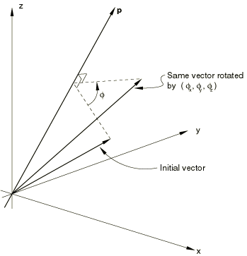
Finite Rotations

The following convention is used for finite rotations in space: Define $ϕ_{x}$ , $ϕ_{y}$ , $ϕ_{z}$ as “rotations” about the global X, Y, and Z-axes (that is, degrees of freedom 4, 5, and 6 at a node). Then define

p_{x} = ϕ_{x} / ϕ, p_{y} = ϕ_{y} / ϕ, p_{z} = ϕ_{z} / ϕ,

where

ϕ = \sqrt{ϕ_{x}^{2} + ϕ_{y}^{2} + ϕ_{z}^{2}} .

The direction $p$ is then the axis of rotation, and $ϕ$ is the angular rotation (in radians) about the axis $p$ according to the right-hand rule (see Figure 2).

The value of $ϕ$ is not uniquely determined. In large-rotation problems where the overall rotation exceeds $2 π$ , any multiple of $2 π$ can be added or subtracted, which may lead to discontinuous output values for the rotation components. If rotations larger than $2 π$ about one axis occur in the positive (negative) direction in Abaqus/Standard, the rotation output varies discontinuously between 0 and $2 π$ ( $- 2 π$ ). In Abaqus/Explicit the rotation output varies in all cases between $- 2 π$ and $2 π$ .

This convention provides straightforward input of kinematic boundary conditions and moments in most cases and simple interpretation of the output. The rotations output by Abaqus represent a single rotation from the reference configuration to the current configuration about a fixed axis. The output does not follow the history of rotation at a node. In addition, this convention reduces to the usual convention for small rotations, even in the case of small rotations superposed on an initial finite rotation (such as might be considered in the study of small vibrations about a predeformed state).

Compound Rotations

Because finite rotations are not additive, the way they must be specified is a bit different from the way other boundary conditions are specified: the increment in rotation specified over a step must be the rotation needed to rotate the node from the configuration at the beginning of the step to that desired at the end of the step. It is not enough to rotate the node over this step to a total rotation vector that would have taken the node into its final configuration if applied on the node in some other initial reference configuration. If an increment of rotation $(Δ ϕ_{x}, Δ ϕ_{y}, Δ ϕ_{z})$ is needed to rotate from the rotation boundary condition ${(ϕ_{x}, ϕ_{y}, ϕ_{z})}^{t}$ at the beginning of the step (and at the end of the previous step) to its final position at the end of the step, the boundary condition must be specified such that the rotation vector is $(ϕ_{x}^{t} + Δ ϕ_{x}, ϕ_{y}^{t} + Δ ϕ_{y}, ϕ_{z}^{t} + Δ ϕ_{z})$ at the end of the step. If the direction of the rotation vector is constant, this method of specifying rotation boundary conditions and the total rotation vector will be the same.

Example

As an example of how to specify compound finite rotations and to interpret finite rotation output, consider the following example of the rotation of a beam.

The beam initially lies along the x-axis. We want to perform the compound rotation, where (Step 1) the beam is rotated by 60° about the z-axis, followed by (Step 2) a 90° spin of the beam about itself, followed by (Step 3) a 90° rotation of the beam about an axis perpendicular to the beam in the x–y plane, such that the beam finishes on the z-axis.

This compound rotation is achieved in three steps with applied rotation vectors $ϕ_{1}$ , $ϕ_{2}$ , and $ϕ_{3}$ , where

\begin{matrix} ϕ_{1} & = ϕ_{1} e_{z} = {\begin{matrix} 0 & 0 & 1.047198 \end{matrix}}^{T}, \\ ϕ_{2} & = ϕ_{2} (\cos ϕ_{1} e_{x} + \sin ϕ_{1} e_{y}) = {\begin{matrix} 0.785398 & 1.360350 & 0 \end{matrix}}^{T}, and \\ ϕ_{3} & = ϕ_{3} (\sin ϕ_{1} e_{x} - \cos ϕ_{1} e_{y}) = {\begin{matrix} 1.360350 & - 0.785398 & 0 \end{matrix}}^{T} . \end{matrix}

For this example $ϕ_{1} = π / 3$ , $ϕ_{2} = π / 2$ , and $ϕ_{3} = π / 2$ . Here $ϕ_{i}$ represents the magnitude of each finite rotation about the (unit length) rotation axis. The rotation vectors above are applied in each of the three steps on the configuration at the beginning of that step. It is most straightforward to prescribe these rotations with velocity-type boundary conditions. For convenience, the default amplitude reference in Abaqus for a velocity-type boundary condition is a constant value of one.

A typical Abaqus step definition for this example, where node 1 is pinned at the origin and the rotation is applied to node 2, is as follows:

STEP, NLGEOM
Step 1: Rotate 60 degrees about the z-axis 
STATIC
BOUNDARY, TYPE=VELOCITY
 2, 4, 5 
 2, 6, 6, 1.047198 
END STEP
** 
STEP, NLGEOM
Step 2: Rotate 90 degrees about the beam axis 
STATIC
BOUNDARY, TYPE=VELOCITY
 2, 4, 4, 0.785398 
 2, 5, 5, 1.36035 
 2, 6, 6 
END STEP
** 
STEP, NLGEOM
Step 3: Rotate beam onto z-axis 
STATIC
BOUNDARY, TYPE=VELOCITY
 2, 4, 4, 1.36035 
 2, 5, 5, -0.785398 
 2, 6, 6 
END STEP

The above method for applying finite-rotation boundary conditions (using a velocity-type boundary condition with the default constant amplitude definition) is strongly recommended. However, if the rotation boundary conditions are applied as displacement-type boundary conditions, the input syntax would change.

The Abaqus/Standard convention for boundary condition specification within a step is to specify the total or final boundary state. In such a case the specified boundary conditions from all of the previous steps must be added to the incremental rotation vector components. The Abaqus/Standard step definitions from above would change to:

STEP, NLGEOM 
Step 1: Rotate 60 degrees about the z-axis 
STATIC
BOUNDARY
 2, 4, 5 
 2, 6, 6, 1.047198 
END STEP
** 
STEP, NLGEOM
Step 2: Rotate 90 degrees about the beam axis 
STATIC
BOUNDARY
 2, 4, 4, 0.785398 
 2, 5, 5, 1.36035 
 2, 6, 6, 1.047198 
END STEP
** 
STEP, NLGEOM
Step 3: Rotate beam onto z-axis 
STATIC
BOUNDARY
 2, 4, 4, 2.145748 
 2, 5, 5, 0.574952 
 2, 6, 6, 1.047198 
END STEP

The boundary conditions in Steps 2 and 3 are the sum of the incremental rotation components plus the rotation boundary conditions specified in the previous steps.

In Abaqus/Explicit references to amplitude definitions should be used such that there are no jumps in displacement across the steps. It is often convenient to use amplitude definitions given in terms of total time for this purpose. The displacement boundary conditions will be applied incrementally based on the increment in the value of amplitude curve over the time increment. Therefore, any sudden jumps in displacement at the beginning of a step introduced either without the amplitude curves or with two amplitude curves is ignored (see Boundary Conditions). The Abaqus/Explicit step definitions for the above example would change to:

AMPLITUDE, TIME=TOTAL TIME, NAME=RAMPUR1
 0., 0., 0.001, 0., 0.002, 0.785398, 0.003, 2.145748
AMPLITUDE, TIME=TOTAL TIME, NAME=RAMPUR2
 0., 0., 0.001, 0., 0.002, 1.36035, 0.003, 0.574952
AMPLITUDE, TIME=TOTAL TIME, NAME=RAMPUR3
 0., 0., 0.001, 1.047198, 0.002, 1.047198, 0.003, 1.047198
STEP
Step 1: Rotate 60 degrees about the z-axis
DYNAMIC, EXPLICIT
 , 0.001
BOUNDARY, AMP=RAMPUR1
 2, 4, 4, 1.0
BOUNDARY, AMP=RAMPUR2
 2, 5, 5, 1.0
BOUNDARY, AMP=RAMPUR3
 2, 6, 6, 1.0
END STEP
**
STEP
Step 2: Rotate 90 degrees about the beam axis
DYNAMIC, EXPLICIT
 , 0.001
END STEP
**
STEP
Step 3: Rotate beam onto z-axis
DYNAMIC, EXPLICIT
 , 0.001
END STEP

The boundary conditions in Steps 2 and 3 are the sum of the incremental rotation components plus the rotation boundary conditions specified in the previous steps.

The Abaqus output of the rotation field at the end of Step 3 is

UR1 = 1.927, UR2 = - 0.5163, UR3 = 1.927 .

We see that none of the individual components of the specified boundary conditions appears in the final rotation output. The final rotation output represents the rotation vector required to obtain the final orientation in a single step.

Suppose that in Step 3 of the previous example we want to apply the rotation vector $ϕ_{3}$ at node 1 instead of at node 2. If the rotation is applied incrementally, the Abaqus/Standard step definition is as follows:

STEP, NLGEOM 
Step 3: Rotate beam onto z-axis 
STATIC
BOUNDARY, TYPE=VELOCITY, OP=NEW
 1, 1, 3 
 1, 4, 4, 1.36035 
 1, 5, 5, -0.785398 
 1, 6, 6 
END STEP

and the Abaqus/Explicit step definition is similar. It is necessary to remove the rotation boundary conditions that are in effect at node 2.

As mentioned previously, using velocity-type boundary conditions is the preferred method for applying finite-rotation boundary conditions. If the rotation boundary condition is to be applied as a displacement-type boundary condition, we must first retrieve the rotation field at node 1 at the end of Step 2. The Abaqus output of this rotation field is

UR1 = 1.412, UR2 = 0.8155, UR3 = 0.8155 .

These rotation vector components must then be added to the incremental rotation vector components we want to prescribe in Step 3. The Abaqus/Standard step definition would change to

STEP
Step 3: Rotate beam onto z-axis 
STATIC
BOUNDARY, OP=NEW
 1, 1, 3 
 1, 4, 4, 2.772 
 1, 5, 5, 0.0301 
 1, 6, 6, 0.8155 
END STEP

and the Abaqus/Explicit step definition would change to:

STEP
Step 3: Rotate beam onto z-axis
DYNAMIC, EXPLICIT
 , 0.001
AMPLITUDE, TIME=STEP TIME, NAME=NODE1UR1
 0., 1.412, 0.001, 2.772
AMPLITUDE, TIME=STEP TIME, NAME=NODE1UR2
 0., 0.8155, 0.001, 0.0301
AMPLITUDE, TIME=STEP TIME, NAME=NODE1UR3
 0., 0.8155, 0.001, 0.8155
BOUNDARY, OP=NEW
 1, 1, 3
BOUNDARY, OP=NEW, AMP=NODE1UR1
 1, 4, 4, 1.
BOUNDARY, OP=NEW, AMP=NODE1UR2
 1, 5, 5, 1.
BOUNDARY, OP=NEW, AMP=NODE1UR3
 1, 6, 6, 1.
END STEP

The boundary conditions are again specified in the Abaqus/Explicit input using amplitude curves to avoid any sudden jump in their values at the beginning of the step. As stated above and in Boundary Conditions, any jumps in the displacement values are ignored and the boundary is maintained at the previous values.

As this last procedure clearly demonstrates, it is simpler to apply finite-rotation boundary conditions as velocity-type boundary conditions rather than as displacement-type boundary conditions. The recommended method of specifying finite-rotation boundary conditions is also described in Boundary Conditions. For further discussion of how finite rotations are accumulated, see Rotation variables.