EOS (Equation of State)

Summary

The equation of state model

can be used to model a material that has only volumetric strength (the material is assumed to have no shear strength) or a material that also has isotropic elastic or viscous deviatoric behavior;
can be used with the metal plasticity or the Johnson-Cook plasticity models except when the choice is ignition and growth;
can be used with the extended Drucker-Prager plasticity models (without plastic dilation) except when the choice is ignition and growth;
can be optionally used with the tensile failure model except when the choice is ideal gas to model dynamic spall or a pressure cutoff.

Table 1. Equation of state model options
Type	Description
Ideal Gas	An ideal gas equation of state.
JWL	A Jones-Wilkins-Lee explosive equation of state.
Ignition and growth	Ignition and growth model equation of state for hock initiation and detonation wave propagation of solid high explosives.
Us-Up	A linear $U_{s} - U_{p}$ equation of state.
Tabular	Provide input in tabular format to model sharp transitions in the pressure-density relationship, such as those induced by phase transformations.
User	Provide general capability for modeling the volumetric response of materials through user subroutine VUEOS.

Ideal Gas

Write an ideal gas equation of state in the form of

p + p_{A} = ρ R (θ - θ^{Z}),

where $p_{A}$ is the ambient pressure, $R$ is the gas constant, $θ$ is the current temperature, and $θ^{Z}$ is the absolute zero on the temperature scale used. It is an idealization to real gas behavior and can model any gases approximately under appropriate conditions (for example, low pressure and high temperature).


Input Data	Description
Gas constant	$R$
Ambient pressure	$p_{A}$

JWL

The Jones-Wilkins-Lee (or JWL) equation of state models the pressure generated by the release of chemical energy in an explosive. This model is implemented in a form referred to as a programmed burn, which means that the reaction and initiation of the explosive is not determined by shock in the material. Instead, the initiation time is determined by a geometric construction using the detonation wave speed and the distance of the material point from the detonation points.

You can write the JWL equation of state in terms of the internal energy per unit mass, $E_{m}$ , as

p = A (1 - \frac{ω_{ρ}}{R_{1} ρ_{0}}) \exp (- R_{1} \frac{ρ_{0}}{ρ}) + B (1 - \frac{ω_{ρ}}{R_{2} ρ_{0}}) \exp (- R_{2} \frac{ρ_{0}}{ρ}) + ω_{ρ} E_{m},

where $A$ , where $B$ , where $R_{1}$ , $R_{2}$ , and $ω$ are user-defined material constants; $ρ_{0}$ is the user-defined density of the explosive; and $ρ$ is the density of the detonation products.

Explosive materials generally have some nominal volumetric stiffness before detonation. It may be useful to incorporate this stiffness when elements modeled with a JWL equation of state are subjected to stress before initiation of detonation by the arriving detonation wave. You can define the predetonation bulk modulus, $Κ_{p d}$ . The pressure is computed from the volumetric strain and $Κ_{p d}$ until detonation, at which time the pressure is determined by the procedure outlined above. The initial relative density ( $ρ / ρ_{0}$ ) used in the JWL equation is assumed to be unity. The initial specific energy $E_{m_{0}}$ is assumed to be equal to the user-defined detonation energy $E_{0}$ .

If you specify a nonzero value of $Κ_{p d}$ , you can also define an initial stress state for the explosive materials.


Input Data	Description
A	User-defined material constant, $A$ .
B	User-defined material constant, $B$
Omega	User-defined material constant, $ω$ , $(ω \geq 0)$
R1	User-defined material constant, $R_{1}$
R2	User-defined material constant, $R_{2}$
Detonation energy density	Positive $E_{0}$
Pre-detonation bulk modulus	Positive $Κ_{p d}$

Currently, no support for specifying coordinates of detonation point is available for this model.

Ignition and growth

The ignition and growth description of the equation of state models shock initiation and detonation wave propagation of solid explosives that react to form gaseous products. It requires the specification of the reaction rate to convert the unreacted solid explosive to reacted gas and the specific heat properties of the reacted gas.

This model assumes the heterogenous explosive to be made of a homogeneous mixture of unreacted solid explosive and the reacted gaseous products. Separate JWL equations of state can be prescribed for each phase at each material point:

p_{s} = {\tilde{F}}_{1 s} (ρ_{s}) - {\tilde{F}}_{1 s} (ρ_{0}) + {\tilde{F}}_{2 s} (ρ_{s}) E_{m s},

p_{g} = {\tilde{F}}_{1 g} (ρ_{g}) + {\tilde{F}}_{2 g} (ρ_{g}) (E_{m g} + E_{d}),

where

{\tilde{F}}_{1 i} (ρ_{i}) = A_{i} (1 - \frac{ω_{i} ρ_{i}}{R_{1 i} ρ_{0}}) \exp (- R_{1 i} \frac{ρ_{0}}{ρ_{i}}) + B_{i} (1 - \frac{ω_{i} ρ_{i}}{R_{2 i} ρ_{0}}) \exp (- R_{2 i} \frac{ρ_{0}}{ρ_{i}})

and

{\tilde{F}}_{2 i} (ρ_{i}) = ω_{i} ρ_{i}, (i = s, g) .

The subscript $s$ refers to the unreacted solid explosive, and $g$ refers to the reacted gas products. $A_{i}, B_{i}, R_{1 i}, R_{2 i},$ and $ω_{i}$ are user-defined material constants used in the JWL equations; $E_{d}$ is the detonation energy; $ρ_{0}$ is the user-defined reference density of the explosive, and $ρ_{i}$ is the density of the unreacted explosive or the reacted products.


Input Data	Description
Detonation Energy	Positive value of detonation energy, $E_{d}$ .

Table 2. Ignition and growth model table
Input Data	Description
As	$A_{s}$
Bs	$B_{s}$
Omega Solid	User material constant $ω_{s}$ , $(ω_{s} \geq 0)$
R1s	$R_{1 s}$
R2s	$R_{2 s}$
Ag	$A_{g}$
Bg	$B_{g}$
Omega Gas	User material constant, $ω_{g}$ ( $ω_{g} \geq 0$ )
R1g	$R_{1 g}$
R2g	$R_{2 g}$

The specific heat of the gas can be specified as a function of temperature and field variables.

Table 3. Gas-specific heat table
Label	Description
Specific Heat	Specific heat of the gas
Use temperature-dependent data	Specifies temperature-dependent stress-strain data. A Temperature field appears in the data table. For more information, see Specifying Material Data as a Function of Temperature and Independent Field Variables.
Number of field variables	Specifies field variable-dependent stress-strain data. A Field field appears in the data table each time the number of field variables is incremented by one. For more information, see Specifying Material Data as a Function of Temperature and Independent Field Variables.

The conversion of unreacted solid explosive to reacted gaseous products is governed by the reaction rate. The reaction rate equation in the ignition and growth model is a pressure-driven rule, which includes three terms:

\frac{d F}{d t} = {\dot{F}}_{i g} + {\dot{F}}_{G_{1}} + {\dot{F}}_{G_{2}} .

These three terms are defined as follows:

\begin{matrix} {\dot{F}}_{i g} & , = I {(1 - F)}^{b} {(\frac{ρ_{s}}{ρ_{0}} - 1 - a)}^{x}, \\ {\dot{F}}_{G_{1}} & , = G_{1} {(1 - F)}^{c} F^{d} {(\frac{p}{p_{r e f}})}^{y}, \\ {\dot{F}}_{G_{2}} & , = G_{2} {(1 - F)}^{e} F^{g} {(\frac{p}{p_{r e f}})}^{z}, \end{matrix}

where $I, G_{1}, G_{2}, a, b, c, d, e, g, x, y$ , and $z$ are reaction rate constants; and $p_{r e f}$ is a reference pressure.

The first term, ${\dot{F}}_{i g}$ , describes hot spot ignition by igniting some of the material relatively quickly but limiting it to a small proportion of the total solid $F_{i g}^{m a x}$ . The second term, ${\dot{F}}_{G_{1}}$ , represents the growth of reaction from the hot spot sites into the material and describes the inward and outward grain burning phenomena; this term is limited to a proportion of the total solid $F_{G_{1}}^{m a x}$ . The third term, ${\dot{F}}_{G_{2}}$ , is used to describe the rapid transition to detonation observed in some energetic materials.

\begin{matrix} {\dot{F}}_{i g} = 0 & if F \geq F_{i g}^{m a x} \\ {\dot{F}}_{G_{1}} = 0 & if F \geq F_{G_{1}}^{m a x} \\ {\dot{F}}_{G_{2}} = 0 & if F \leq F_{G_{2}}^{m i n} \end{matrix}

The various bounds that determine when the reaction rate is zero satisfy

0 \leq F_{i g}^{\max} \leq F_{G 1}^{\max} \leq F_{G 2}^{\min} \leq 1.0

.

Table 4. Reaction rate model
Input Data	Description
I	User material constant $I$ ( $I \geq 0$ )
a	Reaction product covolume, $a$ ( $a > 0$ )
b	Exponent on unreacted fraction in the ignition term, $b$
x	Ignition term exponent, $x$
G1	First burn rate coefficient, $G_{1}$ ( $G_{1} \geq 0$ )
c	Exponent on the unreacted fraction in the growth term, $c$
d	Exponent on the reacted fraction in the growth term, $d$
y	Pressure exponent in the growth term, $y$
G2	Second burn rate coefficient, $G_{2}$ ( $G_{2} \geq 0$ )
e	Exponent on the unreacted fraction in the completion term, $e$
g	Exponent on the reacted fraction in the completion term, $g$
z	Pressure exponent in the completion term, $z$
Fig Max	Initial reacted fraction, $F_{i g}^{\max}$ ( $0 \leq F_{i g}^{\max} \leq 1.0$ )
FG1 Max	Maximum reacted fraction for the growth term, $F_{G 1}^{\max}$ ( $0 \leq F_{G 1}^{\max} \leq 1.0$ )
FG2 Min	Minimum reacted fraction for the completion term, $F_{G 2}^{\min}$ ( $0 \leq F_{G 2}^{\min} \leq 1.0$ )
Reference Pressure	Positive reference pressure, $p_{r e f}$ with default set to 1.0

Us - Up

The Us - Up options allow you to define the Mie-Grüneisen equation of state:

p_{H} = \frac{ρ_{0} {c_{0}^{2} η}_{}}{{(1 - s η)}^{2}},

where $c_{0}$ and $s$ define the linear relationship between the shock velocity, $U_{s}$ , and the particle velocity, $U_{p}$ , as follows:

U_{s} = {c_{0} + s U}_{p} .

The reference density, $ρ_{0}$ , is the material Density, which must be entered separately from the EOS behavior.


Input Data	Description
C0	Reference sound speed.
S	Slope of the $U_{s} - U_{p}$ curve.
Gamma0	Grüneisen ratio.

Tabular

The tabulated equation of state provides flexibility in modeling the hydrodynamic response of materials that exhibit sharp transitions in the pressure-density relationship, such as those induced by phase transformations. The tabulated equation of state is linear in energy and assumes the form

p = f_{1} (ε_{v o l}) + ρ_{0} f_{2} (ε_{v o l}) E_{m},

where $f_{1} (ε_{v o l})$ and $f_{2} (ε_{v o l})$ are functions of the logarithmic volumetric strain $ε_{v o l}$ only, where $ε_{v o l} = \ln (ρ_{0} / ρ)$ , and $ρ_{0}$ is the reference density.

You can specify the functions $f_{1} (ε_{v o l})$ and $f_{2} (ε_{v o l})$ directly in tabular form. The tabular entries must be given in descending values of the volumetric strain; that is, from the most tensile to the most compressive states. The app will use a piecewise linear relationship between data points. Outside the range of specified values of volumetric strains, the functions are extrapolated based on the last slope computed from the data.

Specify at least two rows of data, and the values you specify must conform to the following criteria:

The $f_{1} (ε_{v o l})$ values must be monotonically increasing.
The values of volumetric strain must be in decreasing order.
The value of $f_{1} (ε_{v o l})$ must be zero when volumetric strain also equals zero.

One row must include a zero volumetric strain value.


Input Data	Description
f1 (N_m2)	$f_{1} (ε_{v o l})$
f2	$f_{2} (ε_{v o l})$
Volumetric Strain	The volumetric strain.

Plastic compaction

The Us - Up and the tabular equation of state models also support irreversible compaction behavior during volumetric response for porous solid materials. Typical applications include modeling compaction of granular materials like partially saturated sand during under water explosion or porous metals like aluminum and iron under dynamic loads.

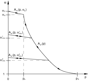
The model requires $p_{e}$ , an elastic limit for pressure below which compaction is assumed to be reversible and $p_{S}$ , a maximum pressure for full compaction. The degree of compaction is expressed in terms of distension $α \geq 1$ ( $α = 1$ at full compaction), with its initial value $α_{0} = 1 / (1 - n_{0})$ in terms of initial porosity $n_{0}$ . The pressure response $p$ as shown in Figure 1 can be separated into a plastic response and several branches of elastic response depending on the deformation history:

p = P (α, α_{m i n}) = {\begin{matrix} P_{p l} (α) & if & α \leq α_{m i n} \\ P_{e l} (α, α_{m i n}) & if & α > α_{m i n} \end{matrix}

Here $α_{\min}$ , is the minimum value of $α$ representing the maximum compaction achieved by the material based on the deformation history experienced so far whenever $p \geq p_{e}$ . In this sense, $α_{\min}$ is a state variable and determines the relevant branch of the elastic response in Figure 1 on elastic unloading or reloading. The plastic portion of the pressure relation is given by

P_{p l} (α) = p_{S} - (p_{S} - p_{e}) {(\frac{α - 1}{α_{e} - 1})}^{\frac{1}{2}} .

Or, equivalently in terms of the inverse relation

A_{p l} (p) = 1 + (α_{e} - 1) {(\frac{p_{S} - p}{p_{S} - p_{e}})}^{2}

Similarly, the elastic portion of the pressure response is given by:

P_{e l} (α, α_{m i n}) = P_{p l} (α_{m i n}) + \frac{(α - α_{m i n})}{{\frac{d {\bar{A}}_{e l}}{d p} |}_{α = α_{m i n}}} .

Again, equivalently the relation is

A_{e l} (p, α_{m i n}) = α_{m i n} + {(p - P_{p l} (α_{m i n})) \frac{d {\bar{A}}_{e l}}{d p} |}_{α = α_{m i n}}

The slope of the elastic pressure response is given by the expression:

\frac{d {\bar{A}}_{e l}}{d p} (α) = \frac{α^{2}}{K_{0}} (1 - \frac{1}{h^{2} (α)}), h (α) = 1 + \frac{(c_{e} - c_{s}) (α - 1)}{c_{s} (α_{0} - 1)},

where $K_{0} = ρ_{s 0} c_{s}^{2}$ is the elastic bulk modulus of the solid material at small nominal strains; $ρ_{s 0}$ is the reference density of the solid; and $c_{s}$ and $c_{e}$ are the reference sound speeds in the solid and virgin (porous) materials, respectively.

In these equations, $α_{e}$ represents the degree of compaction $α_{\min}$ at which the material first experiences irreversible behavior. This parameter is internally calculated by specifying the following nonlinear equation in $α_{e}$ .

P_{e l} (α_{0}, α_{e}) = 0 = P_{p l} (α_{e}) + \frac{(α_{0} - α_{e})}{{\frac{d {\bar{A}}_{e l}}{d p} |}_{α = α_{e}}} .

If the solid is modeled with the Us - Up model, $c_{s}$ is equal to the reference sound speed, $c_{0}$ , which is user specified. On the other hand, if the solid phase is modeled using the tabulated equation of state, $c_{s}$ is computed from the initial bulk modulus and reference density of the solid material, $c_{s} = \sqrt{K_{0} / ρ_{s 0}}$ . In this case the reference density is required to be constant; it cannot be a function of temperature or field variables.


Input Data	Description
Ce	Positive porous material sound speed $c_{e}$ with $c_{e} \leq c_{s}$
n0	$n_{0}$ , $(0 \leq n_{0} \leq 1.0)$
pe	Positive value $p_{e}$
pS	Positive value $p_{S}$ with $p_{e} < p_{s}$

User

The user option provides a general capability to specify pressure $p$ as a function of current density $ρ$ and internal energy per unit mass $E_{m}$ through the user subroutine VUEOS .


Input Data	Description
User defined material parameters	User defined material parameters to calculate pressure as a function of current density and internal energy per unit mass.