Analyze the Results | ||
| ||
-
From the
Standard section of the
action bar,
click
Feature Manager
 .
.
-
From the
Plots
 tab, double-click the
Temperature.1 row.
tab, double-click the
Temperature.1 row.
Tip: You can also select plots from the tree. Press F3 to display the tree if it is not visible, then click Temperature Field Plots from the Results section of the tree. The temperature plot opens in Physics Results Explorer, but the casing obscures our view of the heat sink and fan. You will need to create a plot sectioning cut to look inside.
-
Create a planar plot sectioning cut by doing the following:
-
From the Display section of the action bar, click Plot Sectioning
 .
A triad appears in the middle of the assembly with the U-Y plane as the default cutting plane.
.
A triad appears in the middle of the assembly with the U-Y plane as the default cutting plane. -
From the context toolbar, click Show section, behind, and in
front of cut
 .
The plot sectioning cut section exposes the interior.
.
The plot sectioning cut section exposes the interior.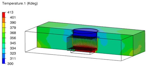
-
From the 3D area, drag a rectangle around the entire model, click
Deactivate cut and close
 to deactivate the planar plot sectioning cut.
-
From the Display section of the action bar, click Plot Sectioning
-
Remove the fluid section from the display by doing the following:
-
From the Display section of the action bar, click Display Group
 .
.
- From the Item options, select Entities and from the Method options, select Sections.
- From the list of Sections, click Fluid Section 1-1.
-
Click
 to remove the fluid section from the display.
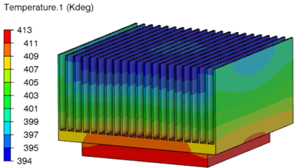
The display shows only the solid sections of the CPU.
-
From the Display section of the action bar, click Display Group
-
From the Display Groups dialog box, click
 to restore the fluid section and click Close.
-
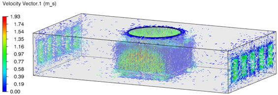
From the Plots
tab of the Feature Manager,
double-click the Velocity Vector.1 row.
-
Review the temperature difference at different points through the chip, the
heat sink, and the enclosure by doing the following:
-
From the Plots section of the action bar, click X-Y Plot from Path
 .
.
- Name the plot Temperature_plot.
-
From the Path options, click
 .
The Path dialog box opens.
.
The Path dialog box opens. - From the Type field, select Point list to create a path from selected points.
-
Click
 , and enter (25, 32, -25),(25, 0,
-25), and (25, 10, 70) in the
coordinates fields.
, and enter (25, 32, -25),(25, 0,
-25), and (25, 10, 70) in the
coordinates fields.
-
Click OK.
The Path dialog box closes, and the app defines the path.
-
From the Templates, select
Temperature, and click
OK.
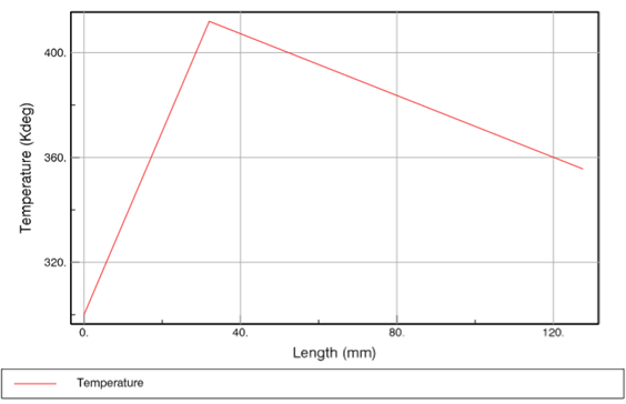
The X-Y plot shows the trend of air temperature through the path created.
The air temperature is 300 K at the inlet of the enclosure, 412 K near the surface of the heat source, and 355 K at the outlet. The increase in the outlet temperature of the air shows that the heat is being taken away from the heat source.
-
From the Plots section of the action bar, click X-Y Plot from Path
Congratulations, you have successfully completed this example!