Analyze the Results

Create sensors to display pertinent variables, and validate the convergence of the simulation. Review and interpret the plots to understand the effects of the duct design on the airflow characteristics.

Sensors filter your output request data for information that you specify, while plots serve as visuals to help you interpret your results in the context of your model. Together, sensors and plots allow you to inspect the quality of a design with respect to a particular variable, such as pressure or flow velocity. You can then use evidence-based decisions to make improvements to the design.

In this example, you place a sensor for mass flow at each duct opening to confirm that the simulation converged properly. You also place a sensor for pressure and velocity at the duct inlet and outlet, respectively. You can use the readings from these sensors to calculate the pressure drop and flow efficiency, which are important factors in the successful design of a duct. A small pressure drop across the duct indicates a low stress on the duct walls, while a consistent flow velocity throughout the duct indicates the duct processes air efficiently. Finally, you plot the pressure, flow velocity, and streamline contours to pinpoint areas of the duct that can be redesigned to optimize the pressure drop and flow velocity.

This task shows you how to:

Create Sensors

  1. Place a sensor at the duct inlet to display the mass flow of air entering the duct.
    1. From the Sensors section of the action bar, click Sensor .
    2. From the Type options, select History.
    3. From the Variable list, select MASSFLOW.
    4. Name the sensor Sensor MASSFLOW_Inlet.
    5. From the Support list, select Output_Inlet.
    6. From the Parameters section, select only Last, and click OK.
  2. Similarly, place a sensor at the duct outlet to display the mass flow of air exiting the duct.
    Expand the Result > Result Of Flow Analysis Case.1 > Sensors node in the tree to find the two mass flow sensors. Expand each sensor's node, and double-click Last to verify that both values are equal and opposite. If they are, mass is conserved and the simulation converged properly.
  3. Place a sensor at the duct inlet to display the last converged average gauge pressure value.
  4. In the tree, expand the pressure sensor's node, and double-click Last.
    The pressure reading at the inlet is approximately 59 N/m2. The pressure at the outlet, which you defined earlier, is 0 N/m2. Therefore, the pressure drop across the duct is 59 N/m2. You can use this value to determine if the design meets its requirements.
  5. Place a sensor at the duct outlet to display the last converged average velocity value.
  6. In the tree, expand the average velocity sensor's node, and double-click Last.
    The average velocity reading at the outlet is approximately 5 m/s. The velocity at the inlet, which you defined earlier, is 5 m/s. Since the values are nearly identical, you can assume that the airflow is unrestricted by the duct's design.

Review and Interpret the Plots

  1. In the Plots window, expand the Plot list and select Gauge Pressure.1 to display the pressure inside the duct.


    As expected, the inlet exhibits a higher pressure than the outlet. The corners of the duct also exhibit high local pressures. This indicates that the design creates too much resistance to the airflow and does not process the air well.

  2. Change your selection to Velocity Vector.1 to display the airflow velocity in vector format.


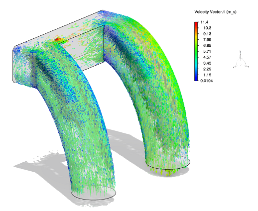
    The velocity is lowest along the boundary layer and in the corners of the duct. While the velocity at the boundary layer is expected, you can improve the airflow resistance in the corners of the duct by smoothing the edges.

  3. Add streamlines to illustrate the airflow through the duct.
    1. From the Results section of the Assistant, click Streamlines .
    2. Expand the Options section, and increase the Thickness to 5 to increase the visibility of the streamlines.
    3. From the Arrows options, select Auto-spaced.
    4. Click OK.
    5. In the Plots window, expand the Plot list and select Velocity.1.


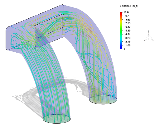
      The streamlines display the flow path from the inlet to the outlet. Airflow is laminar at the inlet but becomes mixed as it passes through the duct. This turbulence is a result of abrupt turns in the duct design. Smoothing the wall's edges and designing fewer turns could reduce the turbulence and pressure drop across the openings.

  4. Save your work.

Congratulations, you have successfully completed this example!