-
From the options at the top of the Calibration Setup
panel, click Execute
 . .
This example uses the default best-fit error measure (the coefficient of
determination, R2) as a convergence criterion measure. This measure
indicates how closely the calibration curve matches the test data points. For
R2, the objective function value is a number between 0 and 1; the
closer to 1, the better the match. The objective function is a measure of the
error between the test data and the predicted material response.
The Calibration History panel appears and provides a plot of
the progress of the calibration, including the value of the objective function
for each iteration.
-
After the calibration completes, review the data in the
Sensitivity column in the Material
model section of the Calibration Setup
panel.
All of the parameters have low
sensitivities
except C10 and g5. However, there is little room for
improvement
because the R2 values are already high.
-
Review the convergence criterion values at the bottom of the
Calibration Setup panel.
Each material response simulated from the calibration demonstrates R 2
values of over
0.99,
indicating that the calibration is representative of the material behavior.
Review the table below to see the sample results of the
calibration.
| Model and Test Data |
Weight |
R2 |
| Strain Rate = 0.01 |
1 |
0.997 |
| Strain Rate = 0.10 |
1 |
0.993 |
| Strain Rate = 1.00 |
1 |
0.998 |
| Strain Rate = 10.0 |
1 |
0.999 |
| Strain Rate = 40 |
0.5 |
0.998 |
-
Review the updated response curve in the Plot panel.
The material response curve is closer to the test data, as shown below. In this
example, the color of the response curves has been changed to green. 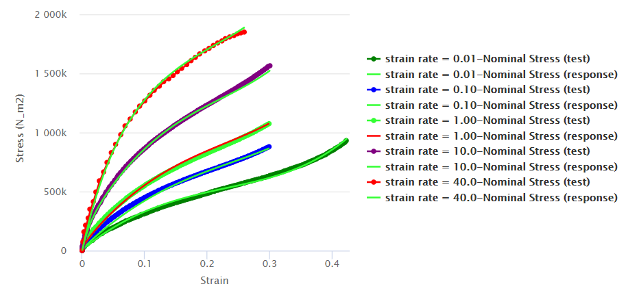 -
Save your work.
|