Perform a Deviation Analysis
You can specify several parameters to perform the deviation analysis.
- From the View section of the action bar, click Customize View
 . . - From the Tools section of the action bar, click Deviation Analysis
 . . - Select the Reference
data and the data To measure:
- Reference data can be a volume, a surface, a plane, a point, a
curve, or a cloud of points.
- To measure data can be clouds of points, points, curves, surfaces,
or volumes.
- When the data To measure are curves, surfaces, or volumes, they are
discretized.
- Multiselection is available:
 is available to hide or show the Reference and the To measure data.
 - Set the computation parameters:
- Determine the discretization Accuracy, available only when at least
one curve, volume, or surface is selected as Reference.
- Select Only Orthogonal to eliminate points
that are not projected orthogonally on the Reference:
- Select Absolute to perform the analysis
with absolute values only.
- When the Reference is a curve, a surface or a body, and for more precise results, select Exact to project the To measure geometry on the Reference exact curve (instead of on its discretization) , or on exact surface (instead of on its tessellation). The projection is either orthogonal or along the chosen direction.
- Select Direction to define a projection direction by picking a plane or
a line.
Notes:
- Right-click
Direction and select the required menu item.
- Or right-click the Robot and select Lock
Privileged Plane Orientation Parallel to Screen and
Robot Direction.
- If you change the direction, do not forget to update the deviation
analysis feature.
- Specify the Visualization parameters:
- Select Spikes to activate the visualization
of the spikes.
- Select Points to change the display to points.
- Click Options to customize the display of
Spikes
and Points.
Use
- Spike scale to change the length of the spikes.
- Point to change the display symbol of points.
- Select Texture to display the deviations
as textures.
Notes:
- Texture is applied to the data To measure.
- The data To measure must be a mesh, a surface or a volume.
- The Render Style must be Shading with
Material. If this is not the case, a message asks you to switch to
this Render Style.
-
Texture mode is available on meshes only, their display
mode being either Flat or Smooth.
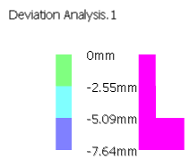
- Texture mode is always available but only triangles with values on their
three vertices are displayed. In the example below, the triangles on the top and
on the left are not displayed in Texture mode.

- There must be a color for each value. The No color and the
Hide
dimmed points options apply to spikes and points visualizations only.
They have no effect on texture mode.
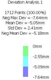
- Select Max values to display the maximum
deviation values (positive and negative) and their locations on the
data To measure.
- Click More>>.
- Define Advanced Parameters and the
Display
Format.
- Select Homogeneous filtering to reduce the number of points of the
data To measure to take into account. A sphere filtering is applied. The parameter represents
the radius of this sphere.
- Select Threshold to remove
points with a
deviation higher than this threshold.
- Select Step when the data to measure are curves, surfaces, oror
volumes. It controls the length of the discretization triangles f surfaces or volumes,
or of the segments for curves. If you do not select this check box and enter a value,
Deviation Analysis computes the step, but in some cases it is
better that you define your own step value.
- Set the Display Format:
- Style: three styles are available:
- Scientific
- Decimal
- Automatic
- Define the Number of significant digits between 1 and 15.
- Click Apply to take any modification into
account.
If Points or Spikes are selected, when you move the pointer over the element To measure, the
deviation value between the point below the pointer and the Reference
data is displayed.
An editable Deviation Analysis.x feature is created. Export the Result as an ASCII File
Provided you have a Virtual to Real Shape Morphing
license, you can export the results of a deviation analysis as an ASCII File.
- Right-click the Deviation Analysis.x feature, and select Export Data.
- Enter an Output directory and File name.
- Optional: Select With distances if you want to export distances information as well.
The exported file can be used in Virtual to Real Shape Morphing. Customize the Color Map
In addition to the Display Format proposed in the dialog box,
you can customize the color map.
- Double-click a color patch.
- In the dialog box, apply No color to this patch, or select another color from
the list.
- Double-click a value.
- Change the value and recompute intermediate values.
- The
Recompute intermediate values check box is displayed once a value
has been changed.
- A warning message is displayed if you enter an inconsistent value.
- Right-click the color map.
- Select
Edit number of colors to define the number of colors to display.
- Select Smooth mode to switch to a smooth mode display.
You cannot modify the colors in Smooth mode. - Select Equalization mode to distribute the values in such a way that
each interval contains the same number of points.
Notes:
- You cannot modify the values in Equalization mode.
- This mode is not always possible (for example concentration of points on one value).
- There is one distribution for the positive values and one for the
negative values.
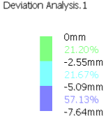
- Select Display, then select the required item:
- All: Selects all the items below (Results, Statistics, Tolerances, Histogram).
- None: None of the items below (Results, Statistics, Tolerances, Histogram)
is selected.
- Results
- Statistics
- Tolerances
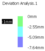
Double-click the tolerance to edit it. - Histogram
You can combine all these options. - Select Hide dimmed points.
Points are dimmed for three reasons:
- They are out of the color map: the max. values are [0,10], you change them to
[0,5]. The points inside [5,10] are dimmed.
- They are inside the tolerance and the option Dim points inside the
tolerance is selected.
- They are outside the tolerance and the option Dim points outside the
tolerance is selected.
- Select Dim points inside the tolerance.
This menu item:
- Is available only if the Tolerances option is selected.
- Dims the points that are within the tolerance.
- Those points can then be hidden with the option Hide dimmed
points.
- Select Dim points outside the tolerance.
This menu item:
- Is available only if the Tolerances option is selected.
- Dims the points that are not within the tolerance.
- Those points can then be hidden with the option Hide dimmed
points.
- Select Reset to restore the default values.
|