Compute Ridges and Valleys
You can lay out ridges and valleys on a terrain.
-
Expand the Ridges and Valleys section and click
Hide/Show all valleys
 and/or
Hide/Show all ridges and/or
Hide/Show all ridges
 to display these
objects on the selected terrain. to display these
objects on the selected terrain.
-
Keep the Extended mode option selected to extend all
ridges/valleys segments to get longer ones and link them together when possible.
By default, the option is selected. Two sliders are available to manage the
extension of the Minimum length (m) and Minimum slope
(%) for valleys and ridges. The minimum value is set by default, in
meters. The distance range computed according to the model and the slope range is from 0
to 100%.
-
To launch computation, click Apply.
A progress bar is displayed during the computation. You can interrupt the treatment
by pressing Escape.
By default, ridges are displayed in orange and valleys in blue. You can change color
by clicking the color segment under the command:  . .
-
Click a valley or a ridge in the 3D area to
display specific information about the selected object.
A contextual toolbar appears in which you use commands to hide it, change its color
or name.
When ridges/valleys are computed, some incorrect or disrupted mesh areas are detected
and displayed in the shape of red overhanging triangles:

A new feature called Terrain Topography.1 is created in the tree. When you leave the command, double-click the feature and the Terrain
Topography Analysis dialog box opens.
-
To hide/show all the ridges and/or valleys, click
 in the
Terrain Topography Analysis dialog box. in the
Terrain Topography Analysis dialog box.
Compute Slopes
You can make steering arrows appear on a terrain to show slope direction.
-
Select a terrain mesh or a polyhedral feature.
-
Expand the Slopes section and click Hide/Show all
maximum slope vectors
 to display slopes
on the selected terrain. to display slopes
on the selected terrain.
A progress bar is displayed during the computation. You can interrupt the treatment
by pressing Escape.
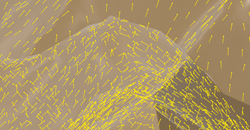
The default color of the arrows is yellow. You can change color by clicking the color
segment under the command. The arrows represent the maximum slope on each triangle of
the input terrain mesh. The slope's segment has a point at its beginning (origin of
the arrow), and not at its end (end of the arrow).
When slopes are computed, some incorrect mesh areas are detected and displayed in the
shape of red overhanging triangles.
A new feature called Terrain Topography.1 is created in the tree. When you leave the command, double-click the feature and the Terrain
Topography Analysis dialog box opens.
-
To hide/show all the slopes, click in the
Terrain Topography Analysis dialog box.
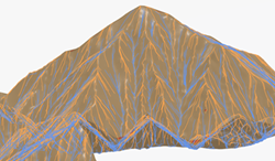
Compute Watershed Segmentation
You can compute and reveal watershed distribution.
A watershed is an area of land that drains all the streams and rainfall to a common outlet
such as a river or a bay. Ridges that separate two watersheds are called the drainage
divide. All the precipitation on opposite sides of a drainage divide will flow into
different drainage basins.
-
Select a terrain mesh or a polyhedral feature.
-
Expand the Watershed Segmentation section and click
 to
display basin division. to
display basin division.
Note:
A message appears telling that the terrain will be hidden to prevent any overlay
with the computation results.
-
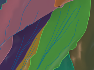
To launch computation, click Apply.
A progress bar is displayed during the computation. You can interrupt the
treatment by pressing Escape. You obtain:
- Colored areas for each basin.
- A black point, called outlet, at the base of each basin.
  Notes:
The water paths do not cross the basins' frontiers (lighter color):
If you click a basin surface, a contextual toolbar appears with the following
information: the name of the basin (editable), depth, Perimeter, area and the
longest Water Path. And two buttons allow you to hide/show the basin or its longest
path and, to change their color.
A new feature called Terrain Topography.1 is created in the tree. When you leave the command, double-click the feature and the Terrain
Topography Analysis dialog box opens.
-
To merge the basins according to a depth value, set a new Depth
threshold in the dedicated box and compute watershed segmentation.
The default value of the depth threshold is 1000mm. If a value is set, this
new value is saved for the next use of Terrain Topography
Analysis. When the value is updated, a preview of merged basins is
displayed in highlighted mode on the terrain. 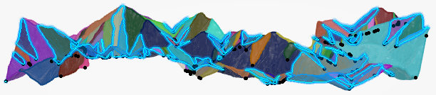 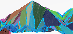 -
To export the watershed data into an xml file, see the last section.
-
To hide/show all the basins, click in the
Terrain Topography Analysis dialog box.
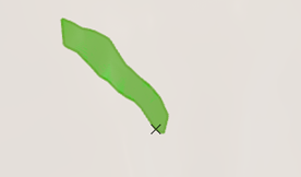
Compute Water Drop Path
You can compute all the trajectories of a water drop starting from a point on the
terrain.
-
Select a terrain mesh or a polyhedral feature.
-
Expand the Water Drop Path section and click
Enable/Disable Water Path
 . .
-
Hover over the terrain surface in the 3D area.
The starting position of the water drop path is given by the pointer. Water
path is displayed in real time: each time the pointer moves, the path is updated. 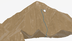 By default,
the water path is displayed in blue. You can change color by clicking the color
segment under the command. -
Click the terrain surface to keep the water path polyline.
You can display several water paths.
A new feature called Terrain Topography.1 is created in the tree. When you leave the command, double-click the feature and the Terrain
Topography Analysis dialog box opens.
-
To remove all the water paths, click
 . .
-
To hide/show all the water drop paths, click in the
Terrain Topography Analysis dialog box.
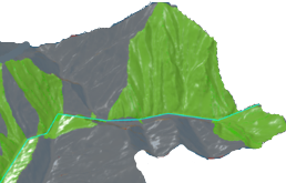
Compute a Catchment Area
You can select a predefined geometry (point(s), polyline, curve or closed polyline)
as an input to display a catchment area. Thus you can see a water drop path on a smaller
portion of the terrain.
This command can be combined with the Watershed segmentation
computation.
-
Select a terrain mesh or a polyhedral feature.
-
Expand the Catchment Area section.
The Compute Catchment Areas from selected objects
 command is
automatically selected. -
To detect water paths in a specific area, select a point, a polyline, a curve or a
closed polyline.
You can select several points to display several water drop areas.
Note:
A message informs you that the terrain transparency will change to allow a better
visibility of the localized catchment area.
-
Optional: To set the depth of the selected areas, change the
Depth threshold value.
This value is also shared with the Watershed segmentation
computation.
-
To launch computation, click Apply.
A progress bar is displayed during the computation. You can interrupt the treatment
by pressing Escape.
The catchment area is the union of all the water drop paths which go through the
input.
The other areas of the terrain are made opaque to provide a better visibility for the
computed area.
Notes:
- To cancel transparency on terrain, do one of the following:
- Hide the catchment areas by clicking .
- Click OK: transparency is cancelled and catchment
areas are still visible.
- Select the terrain Properties and edit the
transparency coefficient in the Graphic tab.
- Watershed segmentation can be executed in parallel. An
advice message appears: it is recommended to hide the segmentation or catchment
area results for better performance.
-
Click the catchment area in the 3D area to
display specific information about it: the name, input type (point, polyline, curve,
closed polyline), perimeter in m, and area in m2 of the catchment area.
You can change its color or name, and hide it by clicking .
A new feature called Terrain Topography.1 is created in the tree. When you leave the command, double-click the feature and the Terrain
Topography Analysis dialog box opens.
-
To open the list of the selected geometry features in a Catchment
Area panel, click
 and, if necessary do the
following: and, if necessary do the
following:
- Select another feature in the tree or in the 3D area and
its name is added to the list.
- Click
 to remove a feature
from the list. to remove a feature
from the list.
- Click
 next to a selected object
for other actions, for example to reframe on it, to hide/show it, to look at its
properties. next to a selected object
for other actions, for example to reframe on it, to hide/show it, to look at its
properties.
-
To export the watershed data into an xml file, see the last section.
-
To hide/show all the catchment areas, click in the
Terrain Topography Analysis dialog box.
Manage Terrain Topography Information
Several actions are available at the bottom of the Terrain Topography
Analysis dialog box to hide/show or reset information. After computing the
watershed segmentation, you can also export the watershed data into an xml file that can be
read in Excel. By default, all basins are exported. If some basins are selected, you export
only on these basins.
-
To hide/show any topography contextual toolbars, click
 . .
-
To reset the color of basins, longest paths, water paths, ridges, valleys or slopes,
click
 . .
-
To export watershed data into an xml file, click
 . .
The following parameters, belonging to the basins, are written in the file:
name, profile, perimeter, area, the length of the longest path, the 3D coordinates of
the lowest point/of the highest point/of the outlet point, and the basin color (RGB
format).
|
 from the