Predicting Prices and Comparing Suppliers

If you study purchase orders for the same category of parts, you can analyze cost drivers and find price models that will help you optimize procurement and sourcing.

Cost drivers may be attributes coming from the parts (extracted from OnePart and defined when installing the application) or attributes related to buying (for instance, the quantity of ordered parts). You can then use the graph to compare different suppliers on the same category of parts and benchmark them for instance (see Compare Suppliers - Use Case).

This task shows you how to:

Create a Price Model
Predict Prices Following a Price Model/Equation
Estimate a Price
Compare Suppliers - Use Case

Create a Price Model

By creating price models, you will be able to reuse existing prices and compare them.

Select a cluster from the Overview page.
Go to the Analytics page.

A graph showing the evolution of prices according to the quantity ordered is displayed. Each blue point on the chart represents a purchase order that can be viewed and opened below the graph.
In the table, define:
- the x and y axis for your variables (here price against ordered quantity)
- the weight for each variable
Select the type of regression analysis you need to perform.
Select > Edit models.
Name your model and click Create model.

Predict Prices Following a Price Model/Equation

You can apply an existing model or equation to your current price analysis.

Select a cluster from the Overview page.
Go to the Analytics page.

A graph showing the evolution of prices according to the quantity ordered is displayed. Each blue point on the chart represents a purchase order that can be viewed and opened below the graph.
Select > Edit models.
Select:
- Load model to load the model containing the table customization
- Load equation to load the corresponding equation (in the form of y = -0.07x + 22.64 for instance).
The graph is updated accordingly.

Estimate a Price

You may need to estimate a price for a part that has not been ordered yet or for or a given quantity of parts.

Select a part or a cluster from the Overview page.
Go to the Analytics page.

A graph showing the evolution of prices according to the quantity ordered is displayed. Each blue point on the chart represents a purchase order that can be viewed and opened below the graph.
In the table, define:
- the x and y axis for your variables
- the weight for each variable
Select the type of regression analysis you need to perform.
In the Prediction column, enter the value that you need to display in the graph (in this example, the price for 15 parts).
Click Predict.

The value is displayed as a yellow sqaure in the graph.

Compare Suppliers - Use Case

In the following example, we will study the price variation found in different suppliers for a given part category (linear brackets).

Go to the Analytics page and begin by filtering on the Linear Bracket category:
Here we will use quantity and volume as cost drivers in the y axis:
We will use linear regression to view our purchase orders and save it as a model for future reference for linear brackets:
Let's now compare suppliers:
- Take a closer look at purchase orders higher than the model price and find the corresponding supplier in the table below the graph.
- Add this supplier as filter.
- Use linear regression to create a model corresponding to the most expensive supplier (here Supplier 28).
Let's do the same for the less expensive supplier (Supplier 8):
- Take a closer look at purchase orders lower than the model price and find the corresponding supplier in the table below the graph.
- Add this supplier as filter.
- Use linear regression to create a model corresponding to the less expensive supplier (here Supplier 8).
We can now load the linear bracket reference model and the equations corresponding to our two suppliers:

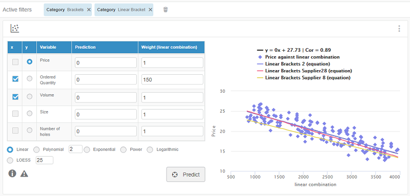
We can see that Supplier 8 is less expensive, even for smaller ordered quantities. For bigger quantities, Supplier 8 and Supplier 28 are close and below the reference model.