About Result Options | ||
| ||
The changes you make to result options for a particular component apply to all plots and other results display for that component.
Display of Plot Sectioning Cuts during View Manipulation
If you have a plot sectioning cut active to display a cross-sectional view of a large or complex model, you might want to hide the cut before you manipulate your view of the model. View manipulations such as rotations, zooms, and panning can impact performance when plot sectioning cuts are active. You can configure the app to hide the view cut whenever you perform any view manipulation for your model.
Symbol Plots
The result options enable you to control the length of vector and tensor arrows for all symbol plots in your session. You can configure arrow size so that all arrows are the same length throughout all symbol plots, or you can display the arrows so that the longer arrows correspond to larger values. For arrows that vary in length, you can specify a maximum vector length as a percentage of the size of your model or using a specific value that is not tied to model size.
Resultant Forces and Moments
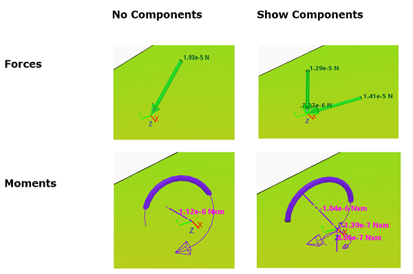
You can display nodal forces or moments computed at the locations selected for each of the resultant sensors in your simulation. You can also choose whether to display the component vectors of forces and moments or to display the Total Force and Total Moment.
The figures below show the resultant sensor glyphs displayed when various options are
enabled or disabled.
Connectors
You can display data associated with the connectors specified in your simulation, including their location, type, descriptive labels, and the local axes used to orient them, if any.
SPH Surface Data
If your simulation includes particles from a smooth particle hydrodynamics (SPH) simulation, you can adjust the grid spacing to change the number of SPH particles that are displayed. Grid spacing depends on particle density and geometry and is the distance between vertices along X-, Y-, and Z-axes of the grid. Grid spacing has four settings: Coarse, Medium, Fine, and Extra Fine. A finer grid provides a smoother surface at the expense of performance in terms of memory and CPU.
You can also change the surface value for which the isosurface is extracted. This value varies between 0 and 1; the default is 0.5.
2D Elements
If your simulation results include planar elements or axisymmetric elements, you can control how these two-dimensional components are rendered to improve your display of the results.
Mirroring Models
When you use mirroring, you reflect the model around one or more planes. When you use patterning, you choose a circular or rectangular pattern to duplicate instances of the original. You can combine the two methods to achieve the desired view of the model.
The duplicated portions from mirroring and patterning are for visualization only. Any numerical representation of results is accurate only for the portion of the model that was analyzed.
You can mirror results using a coordinate system and up to three planes (XY, YZ, and XZ). The mirrored portion is a visualization tool only; any numerical representation of results is accurate only for the portion of the model that was analyzed.
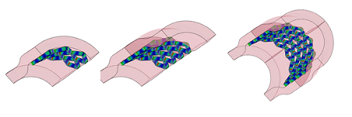
The following figure (below, at left) shows one quarter of a stent in a blood vessel as it was
modeled for analysis. The same model is mirrored about the XZ plane (below, middle)
and the YZ plane (below, right) to display the stent and blood vessel as it would
appear on cross-section.
If you now apply mirroring about the XZ plane, all three symmetry planes (XY, YZ, and XZ) are
enabled, and you can view the complete stent as it would appear in the dilated blood
vessel. 
Patterning Models
You can display results in rectangular or circular patterns to duplicate instances of the original. In a rectangular pattern, you specify the number of instances to display in the X-, Y-, and Z-axis direction, and the distance to offset each one. In a circular pattern, you select an axis of rotation about which to create a specified number of instances of the model. In addition, you specify the total angle within which the instances are equally spaced. For example, you could evenly distribute two instances within 270° or six instances within 180°.
In the example below, two instances of the model are shown evenly distributed in a 360°
circular pattern about the Z-axis.
The patterned portion is a visualization tool only; any numerical representation of results is accurate only for the portion of the model that was analyzed.
Assigning the Order of Operations
When using a combination of mirrors and patterns, you can specify the order of operations to produce the desired view. For example, in a sequence of operations, you can choose to enforce mirroring before a rectangular pattern, or a circular pattern before mirroring, or any permutation of all three model symmetry options.