Acoustic-acoustic tie constraint in three dimensions

This example illustrates and verifies the use of the tie constraint in a simple three-dimensional acoustic system, using several procedures.

This page discusses:

ProductsAbaqus/StandardAbaqus/Explicit

Problem description

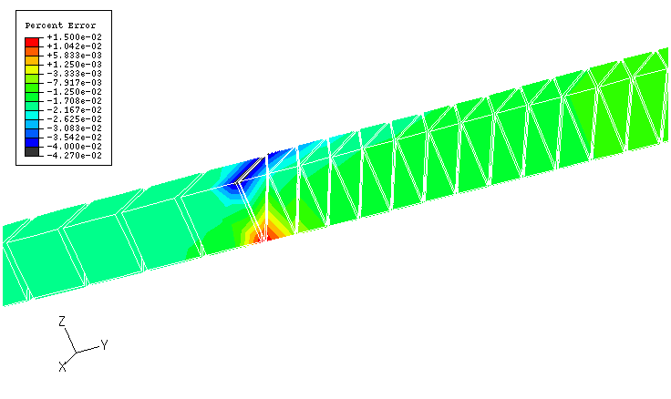
This problem examines the natural frequencies of and the steady-state and transient wave propagation in a rectangular duct 20 meters in length and 1 meter square in cross-section. Figure 1 shows the three-dimensional test mesh. The model is split into two regions: one region has AC3D15 triangular prism elements (AC3D6 triangular prism elements in Abaqus/Explicit), while the other has AC3D4 tetrahedral elements. Both regions are 10 meters long and are connected through tie constraints. Both regions are made of an acoustic material with a bulk modulus of 0.142 MPa and a density of 1.21 kg per cubic meter. The surface on the AC3D15 (AC3D6 in Abaqus/Explicit) side is defined as the secondary surface in the constraint pair.

Loading

The frequency analysis uses no imposed boundary conditions or loads; in acoustic analysis this corresponds to rigid-wall (Neumann) boundary conditions on all exterior surfaces.

In the steady-state dynamic analyses the nodes on the right (unconstrained) end of the AC3D4 mesh are excited using a boundary condition on degree of freedom 8. A plane wave absorbing impedance condition is imposed on the left end of the AC3D15 domain.

In the transient dynamic problems the same boundary condition is applied but with a sinusoidal amplitude. The plane wave condition is imposed here, in the same manner as for the steady-state dynamic analyses.

Results and discussion

The calculated frequencies obtained from the frequency analysis correspond to analytic values, indicating that the constraint transmits the pressure between the mesh regions correctly.

Direct-solution steady-state dynamic analyses are performed at selected frequencies from 5 to 100 Hz. Figure 2 shows the percentage error in the variable POR (pressure field magnitude) at 20 Hz. The mesh is viewed from the point of view opposite to that of Figure 1 to show the area of maximum error. The errors in the vicinity of the constraint are on the order of hundredths of a percent; the response in other regions of the mesh is more accurate.

In the dynamic problem the Abaqus/Standard analysis uses a fixed time increment of 0.0005 seconds. Figure 3 and Figure 4 show the variable POR (pressure magnitude) at a time of 0.04 seconds, shortly after the wavefront has crossed the tie boundary between the tetrahedra and the wedges. The tie constraints introduce minimal distortion and error in the solution.

Figures

Figure 1. Mesh configuration.

Figure 2. Pressure magnitude error at 20 Hz, using a direct-solution steady-state dynamic procedure.

Figure 3. Pressure magnitude at 0.04 seconds, using a dynamic procedure.

Figure 4. Pressure magnitude at 0.04 seconds, using an explicit dynamic procedure.