Test of ORNL plasticity theory under biaxial loading

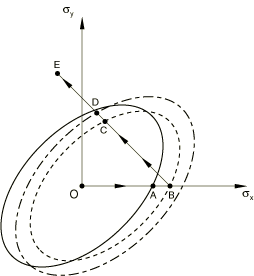
The case is set up with the same geometric and virgin material model as in Case 2 in Uniformly loaded, elastic-plastic plate. The plate is first loaded elastically to the virgin yield surface in the x-direction and then loaded into the plastic range in uniaxial tension in the x-direction to a stress, ${\sigma }_0$, of 276 MPa (40000 lb/in²). Biaxial loading then follows, with ${\sigma }_x$ and ${\sigma }_y$ prescribed, as shown in Figure 1, so that ${\sigma }_y={\sigma }_0-{\sigma }_x$. This loading is defined by an amplitude curve (Amplitude Curves). Abaqus reads in two files (ORNL2.AMP and ORNL3.AMP) of values, which are calculated in the small program AMP (see ornlbiaxialload_ampdata.f).

An “exact” solution is developed by first defining the total strain rates, $d{\epsilon }_x$ and $d{\epsilon }_y$, as functions of the stress rates $d{\sigma }_x$ and $d{\sigma }_y$. The resulting rate equations are then integrated numerically with high accuracy to give a reference solution.

Ziegler's kinematic hardening gives, under isothermal conditions,

where

where ${\sigma }^0$ is the yield stress and

where C is the slope of the stress versus plastic strain curve under uniaxial loading conditions.

Under plane stress conditions (${\sigma }_z=0$) and with ${\sigma }_{xy}=0$,

and

where $A=E/\left(1-{\nu }^2\right)$ and $B=E\nu /\left(1-{\nu }^2\right).$

Hence,

and

where $P=A{n}_x+B{n}_y$, $Q=B{n}_x+A{n}_y.$

The stress rate-strain rate relation is, therefore,

where $\tilde{A}=A-P^2/d$, $\tilde{B}=B-PQ/d$, and $\tilde{C}=A-Q^2/d.$

Inverting this relationship gives the total strain rates as

The center of the yield surface translates according to Ziegler's kinematic hardening rule, so that

where

Hence,

and the translation rate at the center of the yield surface is given in components by

Given the values of the variables ${\sigma }_x$, ${\sigma }_y$, ${\epsilon }_x$, ${\epsilon }_y$, ${\alpha }_x$ and ${\alpha }_y$, at the beginning of the increment, together with the prescribed stress increments $d{\sigma }_x$ and $d{\sigma }_y$, the total strain rate equation and the translation rate equation for the center of the yield surface provide the values of $d{\epsilon }_x$, $d{\epsilon }_y$, $d{\alpha }_x$, and $d{\alpha }_y$.

A small program for calculating the required variables is given in ornlbiaxialload_exact.f. The main program provides prescribed stress increments $\mathrm{\Delta }{\sigma }_x$ and $\mathrm{\Delta }{\sigma }_y$ equal to those used in the finite element analysis. Each of these increments is then split into 1000 subincrements, and the total strain rate equation and the translation rate equation for the center of the yield surface are integrated over each subincrement to provide virtually exact values of $\mathrm{\Delta }{\epsilon }_x$ , $\mathrm{\Delta }{\epsilon }_y$ , $\mathrm{\Delta }{\alpha }_x$ , and $\mathrm{\Delta }{\alpha }_y$ , corresponding to the prescribed values of $\mathrm{\Delta }{\sigma }_x$ and $\mathrm{\Delta }{\sigma }_y$ used in the analysis. In each of the subincrements, a test is made to determine if $\mathit{\alpha }:d{\mathit{\epsilon }}^{pl}<0.$ When this test is satisfied, the yield surface is expanded from the virgin properties to the 10th cycle properties so that ${\sigma }^0$ is increased from its virgin value of 207 MPa (30000 lb/in²) to its 10th cycle value of 234 MPa (34000 lb/in²). This value of ${\sigma }^0$ is used in each subincrement following the initial satisfaction of the test $\mathit{\alpha }:d{\mathit{\epsilon }}^{pl}<0$ , according to the ORNL plasticity algorithm.

References

1. Nuclear Standard NE F9–5T, Guidelines and Procedures for Design of Class 1 Elevated Temperature Nuclear System Components, USDOE Technical Information Center, Oak Ridge, Tennessee, March 1981.