Wave propagation in an infinite medium

This example verifies the effectiveness of the infinite element (quiet boundary) formulation in dynamic applications. The problem is similar to that analyzed by Cohen and Jennings (1983).

This page discusses:

ProductsAbaqus/StandardAbaqus/Explicit

Problem description

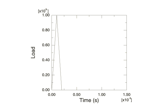
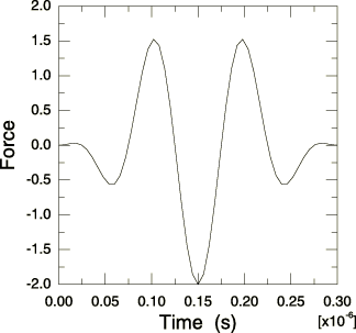
The problem is an infinite half-space (plane strain is assumed) subjected to a vertical pulse line load (see Figure 1). A vertical plane of symmetry is used so that only half the configuration is meshed. Two load cases are considered: a vertical pulse load with a triangular amplitude variation (see Figure 2) and a vertical pulse load in the form of a 10 MHz raised-cosine function, 1-sin(ωt/3)cos(ωt), with an amplitude of 1 GPa and a period of 0.3μs (see Figure 9). A raised-cosine function was chosen because its frequency content has a Gaussian distribution about its center frequency, ω.

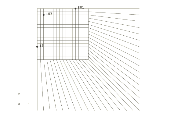
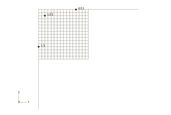
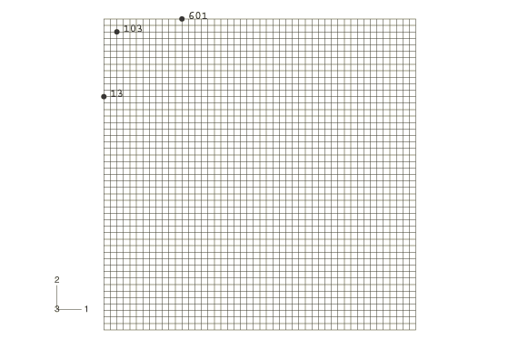
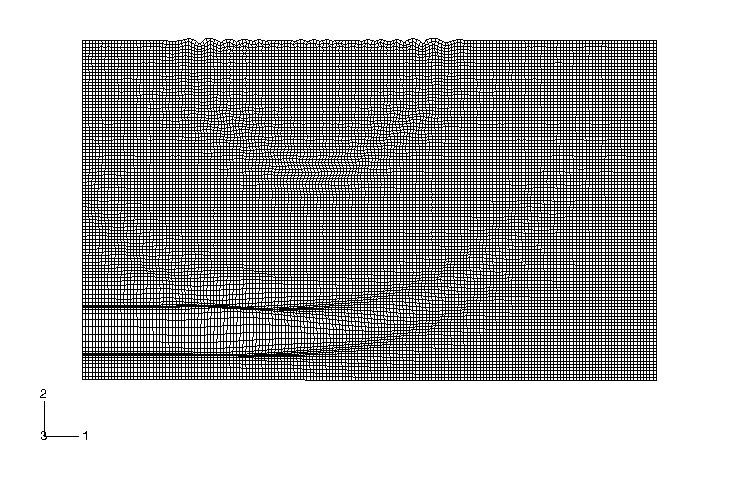
Three meshes are used for load case 1: a small finite/infinite element (quiet boundary) mesh of 16 × 16 CPE4R finite elements plus 32 CINPE4 infinite elements, as shown in Figure 3; a small finite element mesh of 16 × 16 CPE4R elements, as shown in Figure 4; and an extended finite element mesh of 48 × 48 CPE4R elements, as shown in Figure 5. The results obtained using the small mesh including infinite element quiet boundaries are compared with those obtained using the extended mesh of finite elements only. Results obtained using the small mesh without the infinite element quiet boundaries are also given to show how the solution is affected by the reflection of the propagating waves. The mesh used for load case 2 consists of 180 × 107 CPE4R finite elements and 287 CINPE4 infinite elements. The finite element meshes are assumed to have free boundaries at the far field and will reflect the propagating waves, while the finite/infinite element meshes model the infinite domain and provide quiet boundaries that minimize reflection of propagating waves back into the mesh. Geometric nonlinearities are not significant in this problem and are ignored.

The material is assumed to be elastic with the following properties:

Property Value
Young's modulus 73 GPa
Poisson's ratio 0.33
density 2842 kg/m3

Material damping and artificial bulk viscosity are not included in the analyses. Based on these material properties, the speed of propagation of longitudinal waves in the material is approximately 6169.1 m/s, and the speed of propagation of shear waves is approximately 3107.5 m/s (see Solid infinite elements). Therefore, the longitudinal waves, which are predominant with the vertical pulse excitation, should reach the boundary of the small mesh used for load case 1 in about 0.324μs, the boundary of the extended mesh in about 0.97μs, and the boundary of the mesh used for load case 2 in about 0.77μs. Load case 1 analyses are run for 1.5μs, so that the waves are allowed to reflect into the finite element meshes that do not have quiet boundaries.

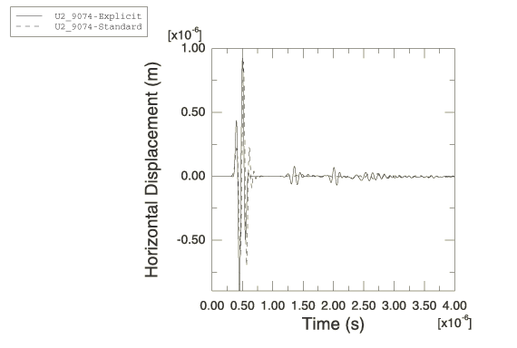
All analyses are performed with both Abaqus/Standard and Abaqus/Explicit.

Results and discussion

The results of load case 1 are shown in the form of time histories of vertical displacements at nodes 13, 103, and 601, as indicated on the meshes. Figure 6 (node 13), Figure 7 (node 103), and Figure 8 (node 601) show the displacement responses. The wave reflection caused by the free boundaries in the small finite element mesh is evident, while the small finite/infinite element quiet boundary mesh largely succeeds in eliminating this reflection. The results obtained with Abaqus/Standard and Abaqus/Explicit agree well.

The wave pattern produced by a distributed load on an infinite half-space is shown in Figure 1. The majority of the energy introduced into the system by the loading is contained in the straight section of the longitudinal wave. The curved wave fronts and the surface waves are produced by the discontinuity at the edge of the distributed load. The same wave pattern can be identified in the deformed configurations of both load cases. In particular, the deformed configuration for load case 2 just prior to the longitudinal wave leaving the lower boundary of the mesh is shown in Figure 10. The contour plots of the vertical and horizontal displacements for load case 2 (see Figure 11 and Figure 12, respectively) show the lower energy shear waves emanating from the edge of the distributed load more clearly.

The time histories of the whole model energies for load case 2 are shown in Figure 13. It can be seen that the kinetic and internal energies remain constant until the longitudinal wave reaches the infinite elements at the mesh boundary. The viscous dissipation time history represents the energy absorbed by the infinite elements. At 1.07μs, when the trailing end of the longitudinal pulse reaches the mesh boundary, most of the energy has been absorbed by the infinite elements. The last wave to exit the mesh should be the shear wave generated by the discontinuity at the edge of the distributed load that travels toward the symmetry axis. It will be reflected by the symmetry axes and travel toward the lower-right corner of the mesh. This should occur at 3.92μs. Any waves remaining in the mesh after this time are due to spurious wave reflection at the infinite boundaries. The kinetic energy associated with these waves is less than 0.2% of the total kinetic energy created by the pulse.

Figure 14 shows the vertical displacement responses of a node positioned 2 mm below the edge of the distributed load. The initial longitudinal pulse reaches the node in 0.324μs. Because the wave is not completely absorbed by the infinite elements, its reflection can be seen on its way back to the surface and again on its return from the surface after it is has been reflected. The response after 2.4μs is due to the shear wave reflecting off the symmetry axis. The shear wave traveling directly downward from the edge of the distributed load does not appear in this plot because its motion is completely in the horizontal direction.

Figure 15 shows the horizontal displacement responses of a node positioned 3.2 mm below the edge of the distributed load. The horizontal component of the longitudinal wave reaches the node in 0.519μs, while the slower traveling shear wave reaches the node at a time of 1.03μs. The response after approximately 1.7μs is due to spurious reflections of the longitudinal and shear waves from the lower boundary as well as the shear wave reflected from the symmetry axes. Again, the results obtained with Abaqus/Standard and Abaqus/Explicit agree well.

Input files

Abaqus/Standard input files

waveprop_fininfmesh.inp

Small finite/infinite element (quiet boundary) mesh of load case 1.

waveprop_smallfinmesh.inp

Small finite element mesh of load case 1.

waveprop_extdfinmesh.inp

Extended finite element mesh of load case 1.

waveprop_3d_fininfmesh.inp

Small finite/infinite element (quiet boundary) mesh of load case 1 in three dimensions.

waveprop_3d_smallfinmesh.inp

Small finite element mesh of load case 1 in three dimensions.

waveprop_3d_extdfinmesh.inp

Extended finite element mesh of load case 1 in three dimensions.

waveprop_prestatic.inp

Contains the analysis in waveprop_fininfmesh.inp preceded by a static step, which is used to verify statics followed by dynamics when using infinite elements.

waveprop_verssd.inp

Contains the analysis to verify STEADY STATE DYNAMICS, DIRECT when using infinite elements.

waveprop_cpe4r_std.inp

CPE4R mesh of load case 2.

waveprop_cpe3_std.inp

The same model meshed with CPE3 elements.

waveprop_ef1.inp

A file that contains the amplitude data for the 10 MHz raised cosine function. This file is read by the two input files listed above.

Abaqus/Explicit input files

waveprop_fininfmesh_exp.inp

Small finite/infinite element (quiet boundary) mesh of load case 1.

waveprop_smallfinmesh_exp.inp

Small finite element mesh of load case 1.

waveprop_extdfinmesh_exp.inp

Extended finite element mesh of load case 1.

waveprop_3d_fininfmesh_exp.inp

Small finite/infinite element (quiet boundary) mesh of load case 1 in three dimensions.

waveprop_3d_smallfinmesh_exp.inp

Small finite element mesh of load case 1 in three dimensions.

waveprop_3d_extdfinmesh_exp.inp

Extended finite element mesh of load case 1 in three dimensions.

waveprop_cpe4r.inp

CPE4R mesh of load case 2.

waveprop_cpe3.inp

The same model meshed with CPE3 elements.

waveprop_ef1.inp

A file that contains the amplitude data for the 10 MHz raised cosine function. This file is read by the two input files listed above.

References

  1. Cohen M. and PCJennings, Silent Boundary Methods for Transient Analysis,” Computational Methods for Transient Analysis, Ed. T. Belytschko and T. R. J. Hughes, Elsevier, 1983.

Figures

Figure 1. Wave pattern caused by a distributed load on an infinite half-space.

Figure 2. Triangular amplitude variation of load case 1.

Figure 3. Small finite/infinite element mesh (quiet boundaries) of load case 1.

Figure 4. Small finite element mesh of load case 1.

Figure 5. Extended finite element mesh of load case 1.

Figure 6. Vertical displacement responses at node 13 (load case 1).

Figure 7. Vertical displacement responses at node 103 (load case 1).

Figure 8. Vertical displacement responses at node 601 (load case 1).

Figure 9. 10 MHz raised-cosine function used for load case 2.

Figure 10. Deformed configuration prior to waves leaving the mesh boundary (load case 2, 0.81μs, displacement magnified by 75%).

Figure 11. Vertical displacement contour at 0.81μs (load case 2).

Figure 12. Horizontal displacement contour at 0.81μs (load case 2).

Figure 13. Whole model energy histories (load case 2).

Figure 14. Vertical displacement response 2 mm below the edge of the load (load case 2).

Figure 15. Horizontal displacement response 3.2 mm below the edge of the load (load case 2).