Problem description
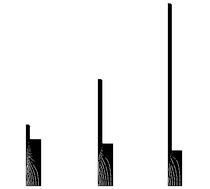
The model configurations for the three analysis cases are shown in Figure 1. Each of the models is axisymmetric and consists of one or more rigid tools and a deformable blank. The rigid tools are modeled as analytical rigid surfaces of connected line segments. All contact surfaces are assumed to be well-lubricated and, thus, are treated as frictionless. The blank is made of aluminum and is modeled as a von Mises elastic-plastic material with isotropic hardening. The Young's modulus is 38 GPa, and the initial yield stress is 27 MPa. The Poisson's ratio is 0.33; the density is 2672 kg/m3.
Case 1: Transient analysis of a backward extrusion
The model geometry consists of a rigid die, a rigid punch, and a blank. The blank is meshed with CAX4R elements and measures 28 × 89 mm. The blank is constrained along its base in the z-direction and at the axis of symmetry in the r-direction. Radial expansion is prevented by contact between the blank and the die. The punch and the die are fully constrained, with the exception of the prescribed vertical motion of the punch. The punch is moved downward 82 mm to form a tube with wall and endcap thicknesses of 7 mm each. The punch velocity is specified using a smooth amplitude so that the response is essentially quasi-static.
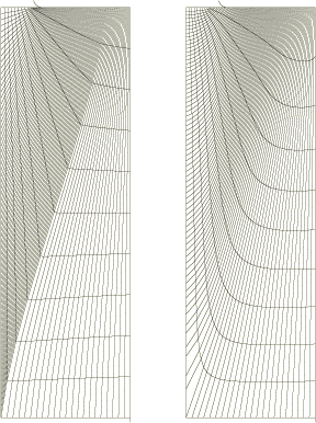
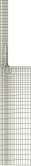
The deformation that occurs in extrusion problems, especially in those that involve flat-nosed die geometries, is extreme and requires adaptive meshing. Since adaptive meshing in Abaqus/Explicit works with the same mesh topology throughout the step, the initial mesh must be chosen such that the mesh topology will be suitable for the duration of the simulation. A simple meshing technique has been developed for extrusion problems such as this. In two dimensions it uses a four-sided, mapped mesh domain that can be created with nearly all finite element mesh preprocessors. The vertices for the four-sided, mapped mesh are shown in Figure 1 and are denoted A, B, C, and D. Two vertices are located on either side of the extrusion opening, the third is in the corner of the dead material zone (the upper left corner of the blank), and the fourth vertex is located in the diagonally opposite corner. A 10 × 60 element mesh using this meshing technique is created for this analysis case and is shown in Figure 2. The mesh refinement is oriented such that the fine mesh along sides AB and DC will move up along the extruded walls as the punch is moved downward.
An adaptive mesh domain is defined that incorporates the entire blank. Because of the extremely large distortions expected in the backward extrusion simulation, three mesh sweeps, instead of the default value of one, are specified for each adaptive mesh increment. The default adaptive meshing frequency of 10 is used. Alternatively, a higher frequency could be specified to perform one mesh sweep per adaptive mesh increment. However, this method would result in a higher computational cost because of the increased number of advection sweeps it would require.
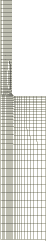
A substantial amount of initial mesh smoothing is performed by increasing the number of mesh sweeps to be performed at the beginning of the step to 100. The initially smoothed mesh is shown in Figure 2. Initial smoothing reduces the distortion of the mapped mesh by rounding out corners and easing sharp transitions before the analysis is performed; therefore, it allows the best mesh to be used throughout the analysis.
Case 2: Transient analysis of a forward extrusion
The model geometry consists of a rigid die and a blank. The blank geometry and the mesh are identical to those described for Case 1, except that the mapped mesh is reversed with respect to the vertical plane so that the mesh lines are oriented toward the forward extrusion opening. The blank is constrained at the axis of symmetry in the r-direction. Radial expansion is prevented by contact between the blank and the die. The die is fully constrained. The blank is pushed up 19 mm by prescribing a constant velocity of 5 m/sec for the nodes along the bottom of the blank. As the blank is pushed up, material flows through the die opening to form a solid rod with a 7 mm radius.
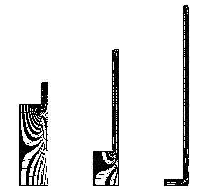
Adaptive meshing for Case 2 is defined in a similar manner as for Case 1. The undeformed mesh configurations, before and after initial mesh smoothing, are shown in Figure 3.
Case 3: Steady-state analysis of a forward extrusion
The model geometry consists of a rigid die, identical to the die used for Case 2, and a blank. The blank geometry is defined such that it closely approximates the shape corresponding to the steady-state solution: this geometry can be thought of as an “initial guess” to the solution. As shown in Figure 4, the blank is discretized with a simple graded pattern that is most refined near the die fillet. No special mesh is required for the steady-state case since minimal mesh motion is expected during the simulation. The blank is constrained at the axis of symmetry in the r-direction. Radial expansion of the blank is prevented by contact between it and the die.
An adaptive mesh domain is defined that incorporates the entire blank. Because the Eulerian domain undergoes very little overall deformation and the material flow speed is much less than the material wave speed, the frequency of adaptive meshing is changed to 5 from the default value of 1 to improve the computational efficiency of the analysis.
The outflow boundary is assumed to be traction-free and is located far enough downstream to ensure that a steady-state solution can be obtained. This boundary is cast as an Eulerian boundary region. A multi-point constraint is defined on the outflow boundary to keep the velocity normal to the boundary uniform. The inflow boundary is defined using an Eulerian boundary condition to prescribe a velocity of 5 m/sec in the vertical direction. Adaptive mesh constraints are defined on both the inflow and outflow boundaries to fix the mesh in the vertical direction. This effectively creates a stationary control volume with respect to the inflow and outflow boundaries through which material can pass.