Problem description
For each analysis case quarter symmetry is assumed; the model consists of a rigid roller and a deformable blank. The blank is meshed with C3D8R elements. The cylindrical roller is modeled as an analytical rigid surface. The radius of the cylinder is 175 mm. Symmetry boundary conditions are prescribed on the right (z=0 plane) and bottom (y=0 plane) faces of the blank.
Coulomb friction with a friction coefficient of 0.3 is assumed between the roller and the plate. All degrees of freedom are constrained on the roller except rotation about the z-axis, where a constant angular velocity of 6.28 rad/sec is defined. For each analysis case the blank is given an initial velocity of 0.3 m/s in the x-direction to initiate contact.
The blank is steel and is modeled as a von Mises elastic-plastic material with isotropic hardening. The Young's modulus is 150 GPa, and the initial yield stress is 168.2 MPa. The Poisson's ratio is 0.3; the density is 7800 kg/m3. The masses of all blank elements are scaled by a factor of 2750 at the beginning of the step so that the analysis can be performed more economically. This scaling factor represents an approximate upper bound on the mass scaling possible for this problem, above which significant inertial effects would be generated.
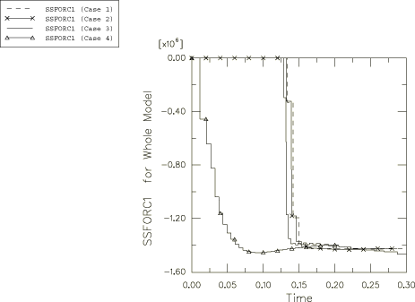
The criteria for stopping the rolling analyses based on the achievement of a steady-state condition is defined. The criteria used require the satisfaction of the steady-state detection norms of equivalent plastic strain, spread, force, and torque within the default tolerances. The exit plane for each norm is defined as the plane passing through the center of the roller with the normal to the plane coincident with the rolling direction. For Case 1 through Case 3 the steady-state detection norms are evaluated as each plane of elements passes the exit plane. Case 4 requires uniform sampling since the initial mesh is roughly stationary due to the initial geometry and the inflow and outflow Eulerian boundaries.
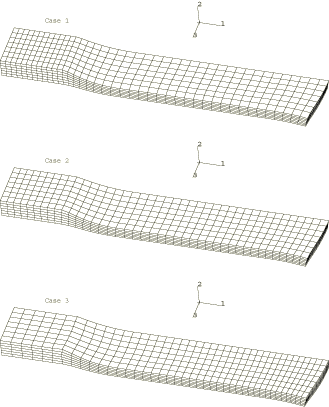
The finite element models used for each analysis case are shown in Figure 2. A description of each model and the adaptive meshing techniques used follows:
Case 1: Transient simulation—pure Lagrangian approach
The blank is initially rectangular and measures 224 × 20 × 50 mm. No adaptive meshing is performed. The analysis is run until steady-state conditions are achieved.
Case 2: Transient simulation—Lagrangian adaptive mesh domain
The finite element model for this case is identical to that used for Case 1, with the exception that a single adaptive mesh domain that incorporates the entire blank is defined to allow continuous adaptive meshing. Symmetry planes are defined as Lagrangian surfaces (the default), and the contact surface on the blank is defined as a sliding surface (the default). The analysis is run until steady-state conditions are achieved.
Case 3: Transient simulation—mixed Eulerian-Lagrangian approach
This analysis is performed on a relatively short initial blank measuring 65 × 20 × 50 mm. Material is continuously drawn by the action of the roller on the blank through an inflow Eulerian boundary defined on the upstream end. The blank is meshed with the same number of elements as in Cases 1 and 2 so that similar aspect ratios are obtained as the blank lengthens and steady-state conditions are achieved.
An adaptive mesh domain is defined that incorporates the entire blank. Because it contains at least one Eulerian surface, this domain is considered Eulerian for the purpose of setting parameter defaults. However, the analysis model has both Lagrangian and Eulerian aspects. The amount of material flow with respect to the mesh will be large at the inflow end and small at the downstream end of the domain. To account for the Lagrangian motion of the downstream end, change the adaptive mesh controls for this problem so that adaptive meshing is performed based on the positions of the nodes at the start of the current adaptive mesh increment. To mesh the inflow end accurately and to perform the analysis economically, the frequency is set to 5 and the number of mesh sweeps is set to 5.
As in Case 2, symmetry planes are defined as Lagrangian boundary regions (the default), and the contact surface on the blank is defined as a sliding boundary region (the default). In addition, the boundary on the upstream end is defined as an Eulerian surface. Adaptive mesh constraints are defined on the Eulerian surface using adaptive mesh constraints to hold the inflow surface mesh completely fixed while material is allowed to enter the domain normal to the surface. An equation constraint is used to ensure that the velocity normal to the inflow boundary is uniform across the surface. The velocity of nodes in the direction tangential to the inflow boundary surface is constrained.
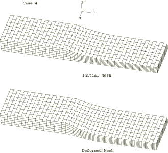
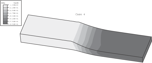
Case 4: Steady-state simulation—Eulerian adaptive mesh domain
This analysis employs a control volume approach in which material is drawn from an inflow Eulerian boundary and is pushed out through an outflow boundary by the action of the roller. The blank geometry for this analysis case is defined such that it approximates the shape corresponding to the steady-state solution: this geometry can be thought of as an “initial guess” to the solution. The blank initially measures 224 mm in length and 50 mm in width and has a variable thickness such that it conforms to the shape of the roller. The surface of the blank transverse to the rolling direction is not adjusted to account for the eventual spreading that will occur in the steady-state solution. Actually, any reasonable initial geometry will reach a steady state, but geometries that are closer to the steady-state geometry often allow a solution to be obtained in a shorter period of time.
As in the previous two cases an adaptive mesh domain is defined on the blank, symmetry planes are defined as Lagrangian surfaces (the default), and the contact surface is defined as a sliding surface (the default). Inflow and outflow Eulerian surfaces are defined on the ends of the blank using the same techniques as in Case 3, except that for the outflow boundary adaptive mesh constraints are applied only normal to the boundary surface and no material constraints are applied tangential to the boundary surface.
To improve the computational efficiency of the analysis, the frequency of adaptive meshing is increased to every fifth increment because the Eulerian domain undergoes very little overall deformation and the material flow speed is much less than the material wave speed. This frequency will cause the mesh at Eulerian boundaries to drift slightly. However, the amount of drift is extremely small and does not accumulate. There is no need to increase the mesh sweeps because this domain is relatively stationary and, by default, adaptive meshing is performed based on the nodal positions of the original mesh. Very little mesh smoothing is required.