Problem description and model definition
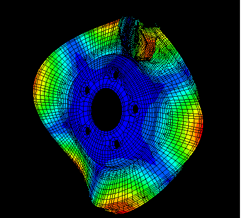
The brake model used in this example is a simplified version of a disc brake system used in domestic passenger vehicles. The simplified model consists of a rotor and two pads positioned on both sides of the rotor. The pads are made of an organic friction material, which is modeled as an anisotropic elastic material. The rotor has a diameter of 288 mm and a thickness of 20 mm and is made of cast iron. The back plates and insulators are positioned behind the pads and are made of steel. In this problem material damping is ignored. The mesh (shown in Figure 1) is generated using C3D6 and C3D8I elements. Contact is defined between both sides of the rotor and the pads using the small-sliding contact formulation. Initially, the friction coefficient is set to zero.
Contact between the rotor and the pads is established initially in the first step by applying pressure to the external surfaces of the insulators. In the next step a rotational velocity of =5 rad/s is imposed on the rotor using the prescribed rotational motion. The imposed velocity corresponds to braking at low velocity. The friction coefficient, , is also increased to 0.3 using a change to friction properties. In general, the friction coefficient can depend on the slip rate, contact pressure, and temperature. If the friction coefficient depends on the slip rate, the velocity imposed by the motion predefined field is used to determine the corresponding value of . The friction coefficient is ramped from zero up to the desired value to avoid the discontinuities and convergence problems that may arise because of the change in friction coefficient that typically occurs when bodies in contact are moving with respect to each other. This issue is described in detail in Static Stress Analysis. The unsymmetric solver is used in this step. At the end of the step a steady-state braking condition is obtained.
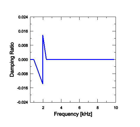
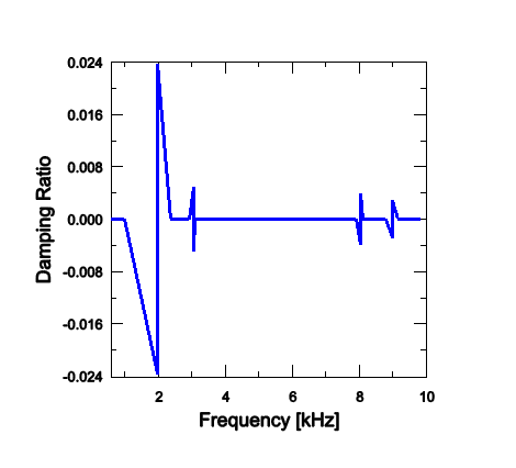
In the next step the eigenvalue extraction procedure is performed in this steady-state condition. Because the complex eigensolver uses the subspace projection technique, the real eigenvectors are extracted first to define the projection subspace. In the eigenvalue extraction procedure the tangential degrees of freedom are not constrained at the contact nodes at which a velocity differential is defined. One hundred real eigenmodes are extracted and, by default, all of them are used to define the projection subspace. The subspace can be reduced by selecting the eigenmodes to be used in the complex eigenvalue extraction step. The complex eigenvalue analysis is performed up to 10 kHz (the first 55 modes).