This example illustrates a typical application of the concrete
damaged plasticity material model for the assessment of the structural
stability and damage of concrete structures subjected to arbitrary loading.
We consider an analysis of the Koyna dam,
which was subjected to an earthquake of magnitude 6.5 on the Richter scale on
December 11, 1967. This problem is chosen because it has been extensively
analyzed by a number of investigators, including Chopra and Chakrabarti (1973),
Bhattacharjee and Léger (1993), Ghrib and Tinawi (1995), Cervera et al. (1996),
and Lee and Fenves (1998).
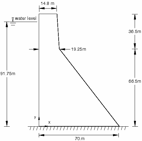
The geometry of a typical non-overflow monolith of the Koyna dam is
illustrated in
Figure 1.
The monolith is 103 m high and 71 m wide at its base. The upstream wall of the
monolith is assumed to be straight and vertical, which is slightly different
from the real configuration. The depth of the reservoir at the time of the
earthquake is
= 91.75 m. Following the work of other investigators, we consider a
two-dimensional analysis of the non-overflow monolith assuming plane stress
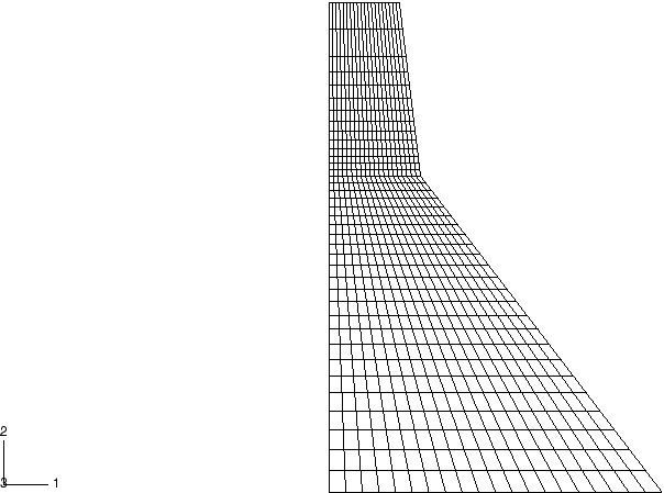
conditions. The finite element mesh used for the analysis is shown in
Figure 2.
It consists of 760 first-order, reduced-integration, plane stress elements (CPS4R). Nodal definitions are referred to a global rectangular
coordinate system centered at the lower left corner of the dam, with the
vertical y-axis pointing in the upward direction and the
horizontal x-axis pointing in the downstream direction.
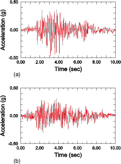
The transverse and vertical components of the ground accelerations recorded
during the Koyna earthquake are shown in
Figure 3
(units of g = 9.81 m sec–2). Prior to the
earthquake excitation, the dam is subjected to gravity loading due to its
self-weight and to the hydrostatic pressure of the reservoir on the upstream
wall.
For the purpose of this example we neglect the dam–foundation interactions
by assuming that the foundation is rigid. The dam–reservoir dynamic
interactions resulting from the transverse component of ground motion can be
modeled in a simple form using the Westergaard added mass technique. According
to Westergaard (1933), the hydrodynamic pressures that the water exerts on the
dam during an earthquake are the same as if a certain body of water moves back
and forth with the dam while the remainder of the reservoir is left inactive.
The added mass per unit area of the upstream wall is given in approximate form
by the expression ,
with ,
where
= 1000 kg/m3 is the density of water. In the
Abaqus/Standard
analysis the added mass approach is implemented using a simple 2-node user
element that has been coded in user subroutine
UEL. In the
Abaqus/Explicit
analysis the dynamic interactions between the dam and the reservoir are
ignored.
The hydrodynamic pressures resulting from the vertical component of ground
motion are assumed to be small and are neglected in all the simulations.
Material properties
The mechanical behavior of the concrete material is modeled using the
concrete damaged plasticity constitutive model described in
Concrete Damaged Plasticity
and
Damaged plasticity model for concrete and other quasi-brittle materials.
The material properties used for the simulations are given in
Table 1
and
Figure 4.
These properties are assumed to be representative of the concrete material in
the Koyna dam and are based on the properties used by previous investigators.
In obtaining some of these material properties, a number of assumptions are
made. Of particular interest is the calibration of the concrete tensile
behavior. The tensile strength is estimated to be 10% of the ultimate
compressive strength (
= 24.1 MPa), multiplied by a dynamic amplification factor of 1.2 to account for
rate effects; thus,
= 2.9 MPa. To avoid unreasonable mesh-sensitive results due to the lack of
reinforcement in the structure, the tensile postfailure behavior is given in
terms of a fracture energy cracking criterion by specifying a
stress/displacement curve instead of a stress-strain curve, as shown in
Figure 4(a).
This is accomplished with the postcracking stress/displacement curve.
Similarly, tensile damage, ,
is specified in tabular form as a function of cracking displacement by using
the postcracking damage displacement curve. This curve is shown in
Figure 4(b).
The stiffness degradation damage caused by compressive failure (crushing) of
the concrete, ,
is assumed to be zero.
Damping
It is generally accepted that dams have damping ratios of about 2–5%. In
this example we tune the material damping properties to provide approximately
3% fraction of critical damping for the first mode of vibration of the dam.
Assuming Rayleigh stiffness proportional damping, the factor
required to provide a fraction
of critical damping for the first mode is given as .
From a natural frequency extraction analysis of the dam the first
eigenfrequency is found to be
= 18.61 rad sec−1 (see
Table 2).
Based on this,
is chosen to be 3.23 × 10⁻³ sec.
Loading and solution control
Loading conditions and solution controls are discussed for each analysis.
Abaqus/Standard
analysis
Prior to the dynamic simulation of the earthquake, the dam is subjected to
gravity loading and hydrostatic pressure. In the
Abaqus/Standard
analysis these loads are specified in two consecutive static steps, using a
distributed load with the load type labels GRAV (for the gravity load) in the first step and HP (for the hydrostatic pressure) in the second step. For the dynamic
analysis in the third step the transverse and vertical components of the ground
accelerations shown in
Figure 3
are applied to all nodes at the base of the dam.
Since considerable nonlinearity is expected in the response, including the
possibility of unstable regimes as the concrete cracks, the overall convergence
of the solution in the
Abaqus/Standard
analysis is expected to be non-monotonic. In such cases automatically setting
the time incrementation parameters is generally recommended to prevent
premature termination of the equilibrium iteration process because the solution
may appear to be diverging. The unsymmetric matrix storage and solution scheme
is activated by specifying an unsymmetric equation solver for the step. This is
essential for obtaining an acceptable rate of convergence with the concrete
damaged plasticity model since plastic flow is nonassociated. Automatic time
incrementation is used for the dynamic analysis of the earthquake, with the
half-increment residual tolerance set to 107 and a maximum time
increment of 0.02 sec.
Abaqus/Explicit
analysis
While it is possible to perform the analysis of the pre-seismic state in
Abaqus/Explicit,
Abaqus/Standard
is much more efficient at solving quasi-static analyses. Therefore, we apply
the gravity and hydrostatic loads in an
Abaqus/Standard
analysis. These results are then imported into
Abaqus/Explicit
to continue with the seismic analysis of the dam subjected to the earthquake
accelerogram. We still need to continue to apply the gravity and hydrostatic
pressure loads during the explicit dynamic step. In
Abaqus/Explicit
gravity loading is specified in exactly the same way as in
Abaqus/Standard.
The specification of the hydrostatic pressure, however, requires some extra
consideration because this load type is not currently supported by
Abaqus/Explicit.
Here we apply the hydrostatic pressure using user subroutine
VDLOAD.
The
Abaqus/Explicit
simulation requires a very large number of increments since the stable time
increment (6 × 10⁻⁶ sec) is much smaller than the total duration of
the earthquake (10 sec). The analysis is run in double precision to prevent the
accumulation of round-off errors. The stability limit could be increased by
using mass scaling; however, this may affect the dynamic response of the
structure.
For this particular problem
Abaqus/Standard
is computationally more effective than
Abaqus/Explicit
because the earthquake is a relatively long event that requires a very large
number of increments in
Abaqus/Explicit.
In addition, the size of the finite element model is small, and the cost of
each solution of the global equilibrium equations in
Abaqus/Standard
is quite inexpensive.
Results and discussion
The results for each analysis are discussed in the following sections.
Abaqus/Standard
results
The results from a frequency extraction analysis of the dam without the
reservoir are summarized in
Table 2.
The first four natural frequencies of the finite element model are in good
agreement with the values reported by Chopra and Chakrabarti (1973). As
discussed above, the frequency extraction analysis is useful for the
calibration of the material damping to be used during the dynamic simulation of
the earthquake.
Figure 5
shows the horizontal displacement at the left corner of the crest of the dam
relative to the ground motion. In this figure positive values represent
displacement in the downstream direction. The crest displacement remains less
than 30 mm during the first 4 seconds of the earthquake. After 4 seconds, the
amplitude of the oscillations of the crest increases substantially. As
discussed below, severe damage to the structure develops during these
oscillations.
The concrete material remains elastic with no damage at the end of the
second step, after the dam has been subjected to the gravity and hydrostatic
pressure loads. Damage to the dam initiates during the seismic analysis in the
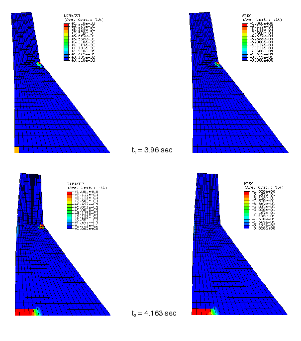
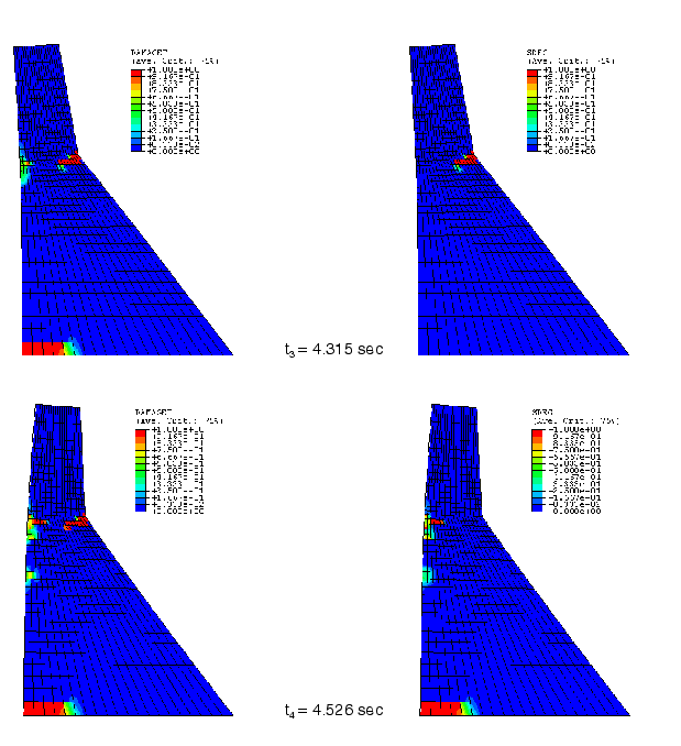
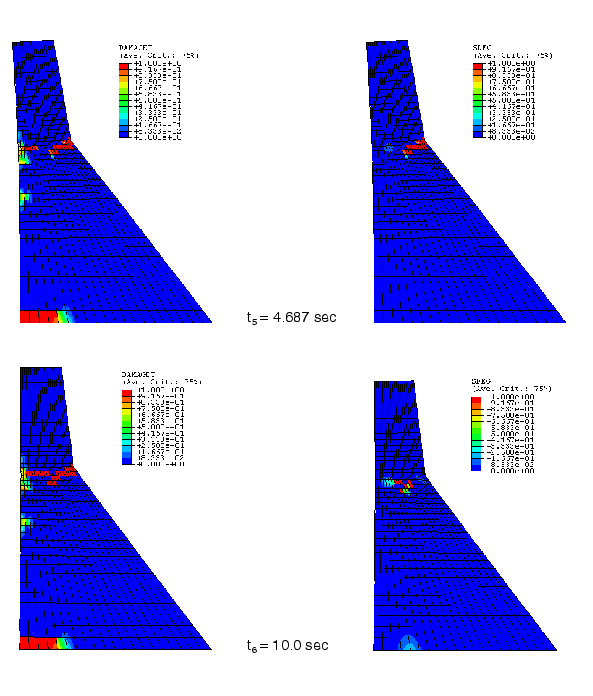
third step. The evolution of damage in the concrete dam at six different times
during the earthquake is illustrated in
Figure 6,
Figure 7,
and
Figure 8.
Times
= 3.96 sec,
= 4.315 sec, and
= 4.687 sec correspond to the first three large excursions of the crest in the
upstream direction, as shown in
Figure 5.
Times
= 4.163 sec and
= 4.526 sec correspond to the first two large excursions of the crest in the
downstream direction. Time
= 10 sec corresponds to the end of the earthquake. The figures show the contour
plots of the tensile damage variable, DAMAGET (or ),
on the left, and the stiffness degradation variable, SDEG (or d), on the right. The tensile damage
variable is a nondecreasing quantity associated with tensile failure of the
material. On the other hand, the stiffness degradation variable can increase or
decrease, reflecting the stiffness recovery effects associated with the
opening/closing of cracks. Thus, assuming that there is no compressive damage
(),
the combination
and
at a given material point represents an open crack, whereas
and
represents a closed crack.
At time ,
damage has initiated at two locations: at the base of the dam on the upstream
face and in the region near the stress concentration where the slope on the
downstream face changes.
When the dam displaces toward the downstream direction at time
,
the damage at the base leads to the formation of a localized crack-like band of
damaged elements. This crack propagates into the dam along the dam–foundation
boundary. The nucleation of this crack is induced by the stress concentration
in this area due to the infinitely rigid foundation. At this time, some partial
tensile damage is also observed on several elements along the upstream face.
During the next large excursion in the upstream direction, at time
,
a localized band of damaged elements forms near the downstream change of slope.
As this downstream crack propagates toward the upstream direction, it curves
down due to the rocking motion of the top block of the dam. The crack at the
base of the dam is closed at time
by the compressive stresses in this region. This is easily verified by looking
at the contour plot of SDEG at time ,
which clearly shows that the stiffness is recovered on this region, indicating
that the crack is closed.
When the load is reversed, corresponding to the next excursion in the
downstream direction at time ,
the downstream crack closes and the stiffness is recovered on that region. At
this time tensile damage localizes on several elements along the upstream face,
leading to the formation of a horizontal crack that propagates toward the
downstream crack.
As the upper block of the dam oscillates back and forth during the remainder
of the earthquake, the upstream and downstream cracks close and open in an
alternate fashion. The dam retains its overall structural stability since both
cracks are never under tensile stress during the earthquake. The distribution
of tensile damage at the end of the earthquake is shown in
Figure 8
at time .
The contour plot of the stiffness degradation variable indicates that, except
at the vicinity of the crack tips, all cracks are closed under compressive
stresses and most of the stiffness is recovered. No compressive failure is
observed during the simulation. The damage patterns predicted by
Abaqus
are consistent with those reported by other investigators.
Abaqus/Explicit
results
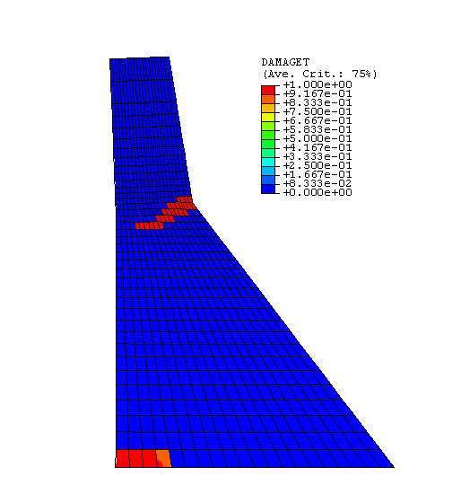
Figure 9
shows the distribution of tensile damage at the end of the
Abaqus/Explicit
simulation. Two major cracks develop during the earthquake, one at the base of
the dam and the other at the downstream change of slope. If we compare these
results with those from the analysis in
Abaqus/Standard
(see
Figure 8
at time ),
we find that
Abaqus/Standard
predicted additional damage localization zones on the upstream face of the dam.
The differences between the results are due to the effect of the dam–reservoir
hydrodynamic interactions, which are included in the
Abaqus/Standard
simulation via an added-mass user element and are ignored in
Abaqus/Explicit.
This is easily verified by running an
Abaqus/Standard
analysis without the added-mass user element. The results from this analysis,
shown in
Figure 10,
are consistent with the
Abaqus/Explicit
results in
Figure 9
and confirm that additional damage to the upstream wall occurs when the
hydrodynamic interactions are taken into account.
Analysis of the post-seismic state of the Koyna Dam; requires import of the
results from koyna_xpl.inp.
References
Bhattacharjee, S.S., and P. Léger, “Seismic
Cracking and Energy Dissipation in Concrete Gravity
Dams,” Earthquake Engineering and Structural
Dynamics, vol. 22, pp. 991–1007, 1993.
Cervera, M., J. Oliver, and O. Manzoli, “A
Rate-Dependent Isotropic Damage Model for the Seismic Analysis of Concrete
Dams,” Earthquake Engineering and Structural
Dynamics, vol. 25, pp. 987–1010, 1996.
Chopra, A.
K., and P. Chakrabarti, “The
Koyna Earthquake and the Damage to Koyna
Dam,” Bulletin of the Seismological Society
of
America, vol. 63, no. 2, pp. 381–397, 1973.
Ghrib, F., and R. Tinawi, “An
Application of Damage Mechanics for Seismic Analysis of Concrete Gravity
Dams,” Earthquake Engineering and Structural
Dynamics, vol. 24, pp. 157–173, 1995.
Lee, J., and G.
L. Fenves, “A
Plastic-Damage Concrete Model for Earthquake Analysis of
Dams,” Earthquake Engineering and Structural
Dynamics, vol. 27, pp. 937–956, 1998.
Westergaard, H.
M., “Water
Pressures on Dams during
Earthquakes,” Transactions of the American
Society of Civil
Engineers, vol. 98, pp. 418–433, 1933.
Tables
Table 1. Material properties for the Koyna dam concrete.
Young's modulus:
E =
31027 MPa
Poisson's ratio:
= 0.15
Density:
= 2643 kg/m3
Dilation angle:
= 36.31o
Compressive initial yield
stress:
= 13.0 MPa
Compressive ultimate
stress:
= 24.1 MPa
Tensile failure stress:
= 2.9 MPa
Table 2. Natural frequencies of the Koyna dam.
Mode
Natural
Frequency (rad sec–1)
Abaqus
Chopra and Chakrabarti
(1973)
1
18.86
19.27
2
49.97
51.50
3
68.16
67.56
4
98.27
99.73
Figures
Figure 1. Geometry of the Koyna dam. Figure 2. Finite element mesh. Figure 3. Koyna earthquake: (a) transverse and (b) vertical ground
accelerations. Figure 4. Concrete tensile properties: (a) tension stiffening and (b) tension
damage. Figure 5. Horizontal crest displacement (relative to ground
displacement). Figure 6. Evolution of tensile damage (Abaqus/Standard);
deformation scale factor = 100. Figure 7. Evolution of tensile damage (Abaqus/Standard);
deformation scale factor = 100. Figure 8. Evolution of tensile damage (Abaqus/Standard);
deformation scale factor = 100. Figure 9. Tensile damage at the end of the
Abaqus/Explicit
simulation without dam–reservoir hydrodynamic interactions; deformation scale
factor = 100. Figure 10. Tensile damage at the end of the
Abaqus/Standard
simulation without dam–reservoir hydrodynamic interactions; deformation scale
factor = 100.