Hydrogen diffusion in a vessel wall section

The problem is shown in Figure 1 and consists of a section of the vessel wall made up of a 200-mm thick base metal and a 5-mm thick weld metal. The problem is one-dimensional, the only gradient being through the thickness of the wall. The purpose of the analysis is to predict the evolution of hydrogen concentration through the wall thickness during cooling caused by a shutdown.

Since the problem is one-dimensional, we use a plane mesh with only one element in the y-direction (see Figure 2). The mesh is graded, with more elements near the interface between the two materials because we expect very high concentration gradients in this vicinity.

The material properties of the two metals given by Fujii et al. (1982) are strongly dependent on temperature and can be written as follows.

Solubility in weld metal:

Diffusivity in weld metal:

Solubility in base metal:

Diffusivity in base metal:

where $\tilde{\theta }$ is temperature in kelvins. These temperature-dependent properties are entered in Abaqus in tabulated form, as shown in the input listings.

The wall is initially at a uniform temperature of 727.5 K (454.4°C), and during the shutdown schedule it cools down to 298.15 K (25.0°C) at a constant rate over a period of 21.5 hours.

The boundary conditions are as follows. Under the initial steady-state conditions the exterior of the weld metal has a hydrogen concentration of 35.85 ppm, which corresponds to a normalized concentration of 0.1225 N^1/2mm⁻¹. Normalized concentration is used as the primary solution variable (continuous over the discretized domain) and is given as the concentration divided by the solubility. The exterior of the base metal has a zero hydrogen concentration. As the cooling period begins, the hydrogen concentration at the exterior of the weld metal is assumed to drop to zero instantaneously.

The problem is run in two parts. The first part consists of a step in which a single increment of steady-state uncoupled mass diffusion analysis is performed with an arbitrary time step to establish the initial steady-state hydrogen concentration distribution corresponding to the initial temperature.

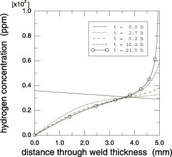
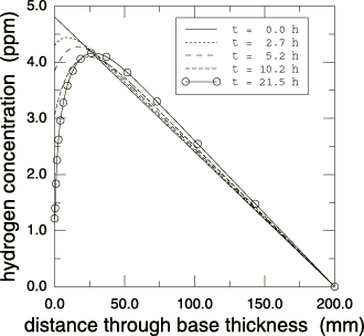
The hydrogen diffusion during cooling is then analyzed in four subsequent mass diffusion transient analysis steps, using automatic time stepping. This need not be done in four separate steps. We do it here because the results given by Fujii et al. (1982), with which we compare the Abaqus results, are presented at four specific times during the transient: 2.7 h (673.15 K, 400.0°C), 5.2 h (623.15 K, 350.0°C), 10.2 h (523.15 K, 250.0°C), and 21.5 h (298.15 K, 25.0°C).

The accuracy of the time integration for the mass diffusion transient analysis steps, during which cooling occurs, is controlled by the DCMAX parameter. This parameter specifies the allowable normalized concentration change per time step. Even in a linear problem such as this, DCMAX controls the accuracy of the solution because the time integration operator is not exact (the backward difference rule is used). In this case DCMAX is chosen as 0.01 N^1/2mm⁻¹, which is a very tight value. This is necessary to obtain an acceptably accurate integration of the concentration because the solubility of the materials decreases significantly (by more than two orders of magnitude in the base metal) as the temperature decreases and, therefore, the changes in concentration become larger for a given change in normalized concentration.

An important issue in transient diffusion problems is the choice of initial time step. As in any transient problem, the spatial element size and the time step are related to the extent that time steps smaller than a certain size may lead to spurious oscillations in the solution and, therefore, provide no useful information. This coupling of the spatial and temporal approximations is always most obvious at the start of diffusion problems, immediately after prescribed changes in the boundary values. For the mass diffusion case the suggested guideline for choosing the initial time increment (see Mass Diffusion Analysis) is

where $\mathrm{\Delta }h$ is a characteristic element size near the disturbance (that is, near the weld metal surface in our case), and D is the diffusivity of the material. For the weld metal in our model we choose a typical $\mathrm{\Delta }h=$ 0.125 mm and we have $D=$ 0.85 mm²/h at the initial temperature, which gives $\mathrm{\Delta }t\ge$ 0.003 h. For the base metal in our model we choose a typical $\mathrm{\Delta }h=$ 1.25 mm and we have $D=$ 4.88 mm²/h at the initial temperature, which gives $\mathrm{\Delta }t\ge$ 0.053 h. Based on these calculations an initial time step of 0.1 h is used, which gives an initial solution with no oscillations, as expected.