Submodeling of a stacked sheet metal assembly

This example shows how the submodeling methodology in Abaqus provides accurate modeling that is more economical than using a globally refined mesh in a single analysis.

This page discusses:

ProductsAbaqus/Standard

Sheet metal stampings stacked and fitted on top of each other and secured together via mechanical fasteners such as bolts or rivets are commonly used in the automotive industry. Examples include seat belt anchors and seating track assemblies. The submodeling capability in Abaqus facilitates economical, yet detailed, prediction of the ultimate strength and integrity of such jointed assemblies. A global model analysis of an assembly is first performed to capture the overall deformation of the system. Subsequently, the displacement results of this global analysis are used to drive the boundaries of a submodeled region of critical concern.

In a finite element analysis of such a structure, shell elements are commonly used to represent the sheet metal stampings. The nodes of each shell typically lie along the mid-plane of the shell thickness. The thickness of the shells is used in the structural calculations but is not taken into account in the contact calculations. Hence, a structure composed of a stack-up of several sheet stampings may have the nodes of each sheet all lying in the same spatial plane. This close proximity creates uncertainty in a submodel analysis since Abaqus will not be able to determine the correct correspondence between the sheets in the submodel and the global model. Therefore, Abaqus provides a capability that allows the user to specify particular elements of the global model that are used to drive a particular set of nodes in a submodel, which eliminates the uncertainty. This capability is demonstrated in this example problem.

Geometry and model

The global model consists of five separate metal stampings meshed with S4R and S3R shell elements. An exploded view of the global finite element model is shown in Figure 1. The stampings are stacked one upon the other by collapsing the configuration in the 3-direction. All the shell elements are 0.5 mm thick, with all nodes positioned at the mid-surface of each shell. The separate meshes are connected together with BEAM-type MPCs between corresponding perimeter nodes on the large bolt holes through each layer. The nodes on the edges of the two small holes at the bottom of Layer 1 are constrained in all six degrees of freedom, representing the attachment point to ground. The translational degrees of freedom of the nodes around the perimeter of Layer 2 are also constrained, representing the far-field boundary condition in that plate.

Several surface definitions are used to model the contact between the various adjacent layers. The contact definitions prevent unwanted penetration between shell element layers. The small-sliding contact formulation is employed. Most of the contact in this problem is between adjacent layers, but there is also direct contact between Layer 2 and Layer 4. To avoid overconstraints, it is important that no point on Layer 4 simultaneously contact Layer 3 and Layer 2; therefore, node-based surfaces are used for the secondary surfaces. This precludes accurate calculation of contact stresses, but that is not important in this case since more accurate contact stresses are obtained in the submodel.

All five stampings are made of steel and are modeled as an elastic-plastic material. The elastic modulus is 207,000 MPa, Poisson's ratio is 0.3, and the yield stress is 250 MPa. The metal plasticity definition includes moderate strain hardening.

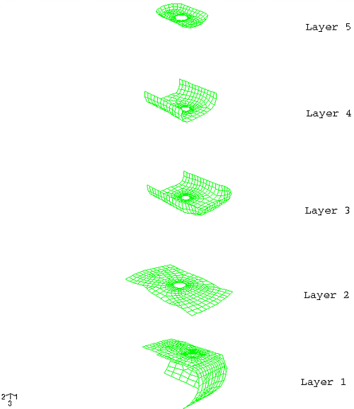
The submodel stampings are truncated versions of the global model, located in the same physical position as the global model. In this case these are the regions of concern for high stresses and potential failure of the joint. The submodel is discretized with a finer mesh than the global model to provide a higher level of accuracy. Figure 2 shows an exploded view of the submodel. Because the stampings in the submodel contain the large bolt holes, the submodel contains BEAM-type MPCs in a manner analogous to that in the global model.

The submodel has several surface definitions and contact pairs to avoid penetration of one stamping into another. The submodel contains no node-based surfaces, however. The contact is modeled as element-based surface-to-surface in each layer.

The material definition and shell thicknesses in the submodel are the same as those in the global model.
Results and discussion

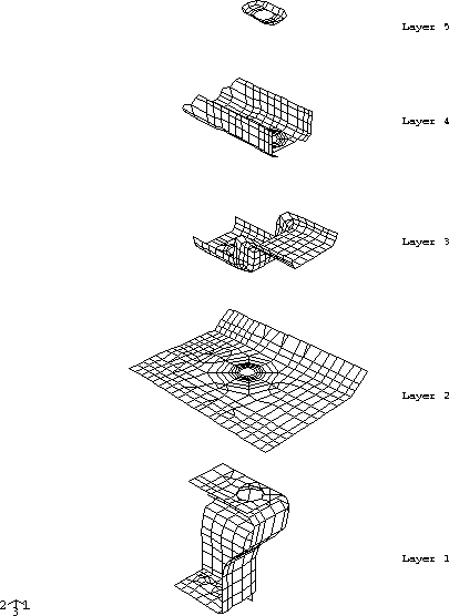
The global model is loaded by enforcing prescribed boundary conditions on the protruding edge of Layer 3. This edge is displaced −5.0 mm in the 1-direction and −12.5 mm in the 3-direction. Figure 3 shows the deformed shape of the global model. The displacements at the nodes are saved to the results file for later use by the submodel analysis.

The submodel driven nodes are loaded using a submodel boundary condition. The perimeter nodes of each layer of the submodel that correspond to a “cut” out of the global geometry are driven by the interpolated nodal displacement results in the global results file. Each driven node set is in a separate shell layer. Therefore, the submodel analysis contains multiple submodels, which designate the global model element sets to be searched for the responses that drive the submodel driven node sets. For example, the driven nodes in submodel Layer 1 (node set L1BC) are driven by the results for the global element set which contains the elements of (global) Layer 1 (element set LAYER1). The driven nodes for Layers 2–4 are specified in a similar way. Because submodel Layer 5 has no driven nodes, only four submodels are required.

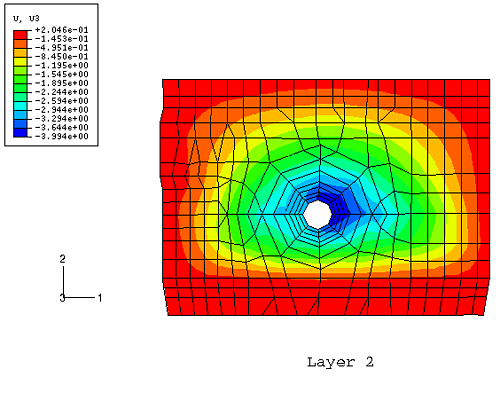
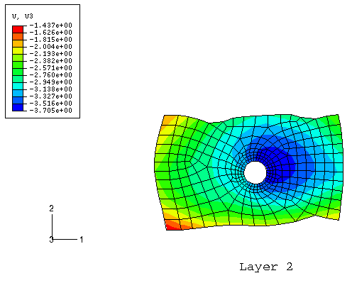
Figure 4 shows the deformed shape of the submodel. Figure 5 and Figure 6 show contour plots of the out-of-plane displacements in Layer 2 for the global model and submodel, respectively. In both cases the displacement patterns are similar; however, the maximum displacement predicted by the global model is about 7.8% larger than that predicted by the submodel.

Figures

Figure 1. Exploded view of global model.

Figure 2. Exploded view of submodel.

Figure 3. Deformed shape of global model.

Figure 4. Deformed shape of submodel.

Figure 5. Out-of-plane displacement in Layer 2, global model.

Figure 6. Out-of-plane displacement in Layer 2, submodel.