User-Defined Mechanical Material Behavior

The subroutine interface has been implemented using Cauchy stress components (“true” stress). For soils problems “stress” should be interpreted as effective stress. The strain increments are defined by the symmetric part of the displacement increment gradient (equivalent to the time integral of the symmetric part of the velocity gradient).

The orientation of the stress and strain components in user subroutine UMAT depends on the use of local orientations (Orientations).

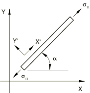
In user subroutine VUMAT all strain measures are calculated with respect to the midincrement configuration. All tensor quantities are defined in the corotational coordinate system that rotates with the material point. To illustrate what this means in terms of stresses, consider the bar shown in Figure 1, which is stretched and rotated from its original configuration, $AB$, to its new position, $A^{\prime }{B}^{\prime }$. This deformation can be obtained in two stages; the bar is first stretched, as shown in Figure 2, and is then rotated by applying a rigid body rotation to it, as shown in Figure 3.

Figure 1. Stretched and rotated bar.

Figure 2. Stretching of bar.

Figure 3. Rigid body rotation of bar.

The stress in the bar after it has been stretched is ${\sigma }_{11}$, and this stress does not change during the rigid body rotation. The $X^{\prime }{Y}^{\prime }$ coordinate system that rotates as a result of the rigid body rotation is the corotational coordinate system. The stress tensor and state variables are, therefore, computed directly and updated in user subroutine VUMAT using the strain tensor since all of these quantities are in the corotational system; these quantities do not have to be rotated by the user subroutine as is sometimes required in user subroutine UMAT.

The elastic response predicted by a rate-form constitutive law depends on the objective stress rate employed. For example, the Green-Naghdi stress rate is used in VUMAT. However, the stress rate used for built-in material models may differ. For example, most material models used with solid (continuum) elements in Abaqus/Explicit employ the Jaumann stress rate. This difference in the formulation will cause significant differences in the results only if finite rotation of a material point is accompanied by finite shear. For a discussion of the objective stress rates used in Abaqus, see Stress rates.

Any material constants that are needed in user subroutine UMAT or VUMAT must be specified as part of a user-defined material behavior definition. Any other mechanical material behaviors included in the same material definition (except thermal expansion and, in Abaqus/Explicit, density) will be ignored; the user-defined material behavior requires that all mechanical material behavior calculations be programmed in subroutine UMAT or VUMAT. In Abaqus/Explicit the density (Density) is required when using a user-defined material behavior.

USER MATERIAL, TYPE=MECHANICAL, CONSTANTS=number_of_constants

USER MATERIAL, TYPE=MECHANICAL, CONSTANTS=number_of_constants
DENSITY

If the user material's Jacobian matrix, $\partial \mathrm{△}\mathit{\sigma }/\partial \mathrm{△}\mathit{\epsilon }$, is not symmetric, the unsymmetric equation solution capability in Abaqus/Standard should be invoked (see Defining an Analysis).

USER MATERIAL, TYPE=MECHANICAL, CONSTANTS=number_of_constants, UNSYMM

If you use a hybrid element with user subroutine UMAT, by default Abaqus/Standard replaces the pressure stress calculated from the stress tensor returned by the user subroutine with that derived from the Lagrange multiplier and modifies the Jacobian appropriately (Hybrid incompressible solid element formulation). This approach is suitable for material models that use an incremental formulation (for example, metal plasticity) but is not consistent with the total formulation that is commonly used for hyperelastic materials. In the latter situation the default formulation may lead to convergence problems. Such convergence problems may be observed, for example, when an almost incompressible nonlinear elastic user material is subjected to large deformations. Abaqus/Standard provides an alternate total formulation that is more appropriate in such situations. The total formulation is consistent with the native almost incompressible formulation used by Abaqus for hyperelastic materials (Hyperelastic material behavior), and works better than the default (incremental) formulation for such cases.

Abaqus/Standard also provides a fully incompressible formulation for use with hybrid elements to define a fully incompressible user material response. The fully incompressible formulation is consistent with the native formulation used by Abaqus for incompressible hyperelastic materials. For the total hybrid formulation it is assumed that the deviatoric and the volumetric responses of the material are decoupled and that the volumetric response can be derived from a strain energy potential function. All the native hyperelastic materials in Abaqus use this assumption. For the incompressible hybrid formulation, it is assumed that the deviatoric stress can be derived from a strain energy potential function.

The total hybrid formulation is useful for an almost incompressible hyperelastic response. The volumetric response of the material is assumed to be defined in terms of an alternate variable, $\widehat{J}$, in place of the volume change, $J$. The alternate variable is made available inside user subroutine UMAT. Further details are discussed in UMAT.

The fully incompressible formulation requires you to define only the deviatoric parts of the stress tensor and the material's Jacobian matrix inside the UMAT. Abaqus/Standard automatically accounts for the pressure stress based on the Lagrange multiplier.

USER MATERIAL, TYPE=MECHANICAL, CONSTANTS=number_of_constants, HYBRID FORMULATION=TOTAL

USER MATERIAL, TYPE=MECHANICAL, CONSTANTS=number_of_constants, 
HYBRID FORMULATION=INCREMENTAL

USER MATERIAL, TYPE=MECHANICAL, CONSTANTS=number_of_constants, 
HYBRID FORMULATION=INCOMPRESSIBLE

Many mechanical constitutive models require the storage of solution-dependent state variables (plastic strains, “back stress,” saturation values, etc. in rate constitutive forms or historical data for theories written in integral form). You should allocate storage for these variables in the associated material definition (see Allocating Space for Solution-Dependent State Variables). There is no restriction on the number of state variables associated with a user-defined material.

The user material subroutines are provided with the material state at the start of each increment, as described below. They must return values for the new stresses and the new internal state variables. State variables associated with UMAT and VUMAT can be output to the output database file (.odb) and results file (.fil) using the output identifiers SDV and SDVn (see Abaqus/Standard Output Variable Identifiers and Abaqus/Explicit Output Variable Identifiers).

Normally the default hourglass control stiffness for reduced-integration elements in Abaqus/Standard and the transverse shear stiffness for shell, pipe, and beam elements are defined based on the elasticity associated with the material (Section Controls, Shell Section Behavior, and Choosing a Beam Element). These stiffnesses are based on a typical value of the initial shear modulus of the material, which may, for example, be given as part of an elastic material behavior (Linear Elastic Behavior) included in the material definition. However, the shear modulus is not available during the preprocessing stage of input for materials defined with user subroutine UMAT or VUMAT. Therefore, you must provide the hourglass stiffness parameters (see Methods for Suppressing Hourglass Modes) when using UMAT to define the material behavior of elements with hourglassing modes.

You must specify the transverse shear modulus for the material (see Defining the Elastic Transverse Shear Modulus) or the transverse shear stiffness for the section (see Choosing a Beam Element or Shell Section Behavior) when using user subroutine UMAT or VUMAT to define the material behavior of beams and shells with transverse shear flexibility. If the transverse shear modulus is specified for a user-defined mechanical material that is associated with shells, Abaqus calls user subroutine UMAT or VUMAT in the data check phase of the analysis to obtain the initial plane stress elastic stiffness. It then computes the transverse shear stiffness by matching the shear response for the case of the shell bending about one axis (see Transverse shear stiffness in composite shells and offsets from the midsurface).

The stable time increment in Abaqus/Explicit is a function of the dilatational wave speed of the material and the characteristic length of the element. By default, the dilatational wave speed is determined automatically by Abaqus/Explicit using a numerical calculation of the effective hypoelastic bulk and shear moduli from the user material's constitutive response. In situations when the user material is highly nonlinear, this calculation may not yield a conservative value of the time increment, leading to unstable behavior. To avoid these situations, you can define the values of the effective bulk and shear moduli directly inside user subroutine VUMAT. These values are then used by Abaqus/Explicit to compute the dilatational wave speed and the stable time increment. For more information, see Stability.

USER MATERIAL, EFFMOD

In Abaqus/Standard user subroutine UMATHT can be used in conjunction with UMAT to define the constitutive thermal behavior of the material. The solution-dependent variables allocated in the material definition are accessible in both UMAT and UMATHT. In addition, user subroutines FRIC, GAPCON, and GAPELECTR are available for defining mechanical, thermal, and electrical interactions between surfaces.

In Abaqus/Explicit user subroutine VUMATHT can be used in conjunction with user subroutine VUMAT to define the constitutive thermal behavior of the material. The solution-dependent variables allocated in the material definition are accessible in both VUMAT and VUMATHT. In addition, user subroutines VFRIC, VFRICTION, VUINTER, and VUINTERACTION are availabe for defining interfacial constitutive behavior.