What's New

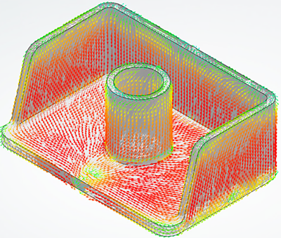
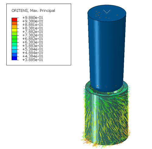
In the example below, the fiber orientation is predicted by an injection molding simulation, as shown in the first figure. The model is then reduced to a simple cylinder, and a rigid rod is added to the model to simulate a service load, as shown in the second figure. The fiber orientation tensor field is mapped from the injection molded part to the reduced model, as shown in second figure.

There is a "weld line" in the cylinder caused by the gate location in the injection molding process; the weld line is the line where the flow fronts meet during the molding process and can result in weakness of the structure. The structural analysis is carried out with Abaqus/Explicit, and a multiscale material is used to model the plastic part. 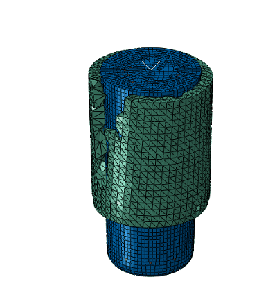Plasticity with ductile damage is specified in the matrix material, and damage evolution is also specified. The third figure shows the deformed shape of the cylinder. As expected, the failure location agrees very well with the location of the weld line.

Two types of plasticity correction are now available in Abaqus: Neuber and Glinka. Both methods apply a correction to the elastic results to capture the effects of local plasticity. The accuracy of the solution is generally quite good when the loading conditions lead to plastic deformation localized in small regions, such as in typical durability load cases. However, a full nonlinear analysis is recommended for loading conditions that lead to extended plastic deformation of the structure. In addition to the general static procedure, the Neuber and Glinka plasticity corrections are supported with the static linear perturbation procedure with multiple load cases, which can further substantially decrease the analysis time.

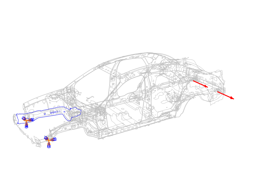
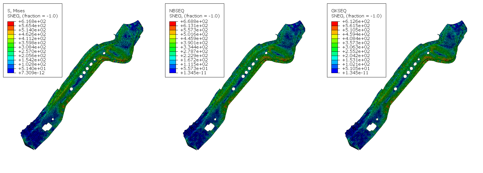
To illustrate the application of the method, consider a Body-in-White (BIW) model of a car subjected to the boundary conditions and loads shown in the first figure (courtesy of the Public Finite Element Model Archive of the National Crash Analysis Center at George Washington University). The stresses and plastic strains in the car body component highlighted in the figure are estimated using the Neuber and Glinka rules with a linear elastic analysis. 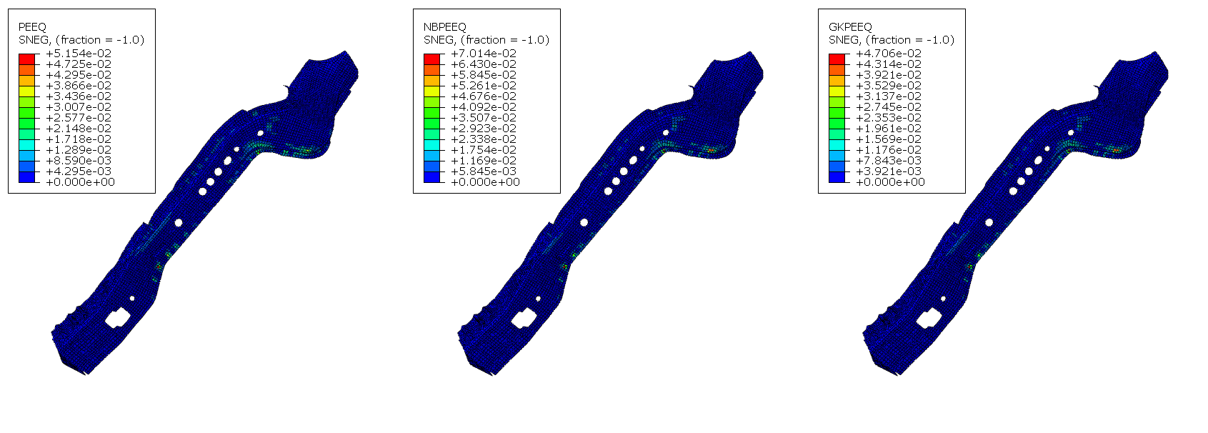The results are compared with those obtained from a full nonlinear elastic-plastic analysis. The stress and plastic strain results are presented in the second and third figures, respectively. The predictions based on plasticity corrections show good agreement with those obtained using a full elastic-plastic analysis, which is expected because plastic deformation is highly localized in small areas of the part. The Neuber's rule overestimates the equivalent stress and plastic strain, which is usually the case. As expected, the Glinka equivalent stress and plastic strain are lower than Neuber’s values. In this case, Glinka's rule slightly underestimates the elastic-plastic results.

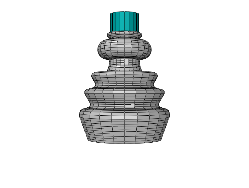
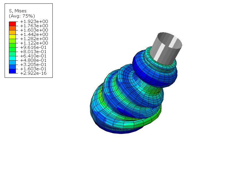
In the example below, the Valanis-Landel material is used to model the rubber sealing in the boot seal assembly shown in the first figure. The shaft is modeled as a rigid body, and contact is specified between the shaft and the inner surface of the seal. The shaft is first rotated 20° about the axis perpendicular to the shaft, and then the angulated shaft moves around the entire circumference. Two analyses were performed with the same Valanis-Landel material defined using two different methods.

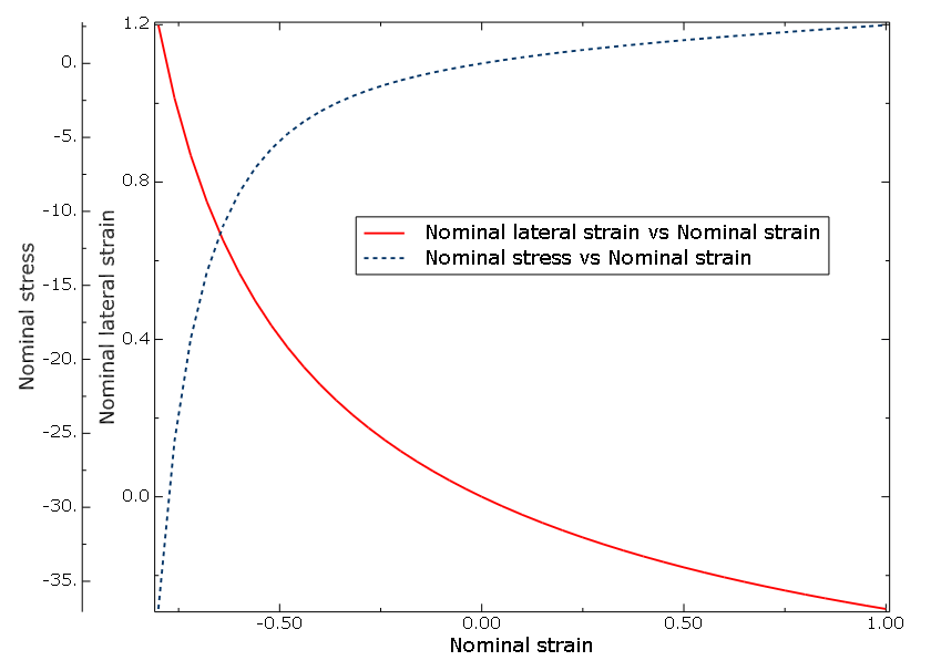
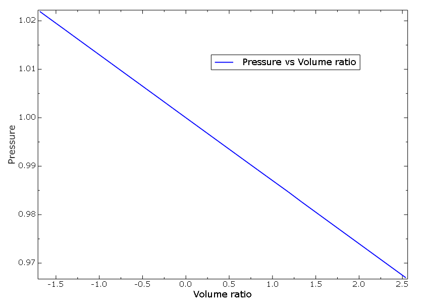
In the first case, the material was defined by providing uniaxial test data with lateral strains shown in the second figure. In the second case, an equivalent material definition using uniaxial test data without lateral strains (dashed line in the second figure) and the volumetric test data (third figure) was used. As expected, the stress results are identical in both cases because the same material response was specified using two different methods. The stress distribution in the seal at the end of the analysis is shown in the fourth figure.

This functionality provides an easy way to extend the linear hardening behavior to a larger strain range. This behavior is often preferable to using a constant value, meaning that the material is perfectly plastic, which might cause convergence problems. Although you can define linear hardening without this functionality by adding one additional data point, it is inconvenient since it requires guessing the range in which the equivalent plastic strain changes during the analysis. In addition, specifying a data point at a very large value of equivalent plastic strain might cause the regularization scheme in Abaqus/Explicit to fail. You can avoid the issues above by specifying linear extrapolation using this new capability.