Discrete element method analysis

This problem contains basic test cases for one or more Abaqus elements and features.

This page discusses:

Elements tested
Features tested
Problem description
Results and discussion
Input files
References
Figures

ProductsAbaqus/Explicit

Elements tested

PD3D

Features tested

Contact interaction between:

two discrete particle elements;
a discrete particle element and a rigid plane; and
JKR and shifted JKR force-displacement relation between contacting discrete particles.

Problem description

This section provides basic verification tests for nonadhesive contact and adhesive contact between discrete particles. For the nonadhesive contact the normal and tangential contact formulations in Abaqus/Explicit are compared with the analytical results based on the Hertzian contact formulation with friction in five tests described in Chung (2011). For the adhesive contact case the results for the JKR and shifted JKR adhesion models in Abaqus/Explicit are compared with analytical solutions.

Table 1. Seven types of tests to verify normal and tangential contact formulation for discrete particle elements.
	Description of contact	Feature tested
Test 1	Elastic head-on collision of two identical spheres	Elastic head-on contact between two spheres
Test 2	Elastic normal impact of a sphere with a rigid plane	Elastic normal contact between a sphere and a plane
Test 3	Oblique impact of a sphere with a rigid plane at a constant normal velocity and an incident angle	Tangential contact between a sphere and a plane
Test 4	Head-on collision of two identical spheres at the same translational speed but with equal and opposite angular speed	Tangential contact between two spheres
Test 5	Head-on collision of two different spheres with different translational and angular velocities	Tangential contact between two spheres
Test 6	Normal adhesive contact between two particles	JKR adhesion between two spheres.
Test 7	Normal adhesive contact between two particles	Shifted JKR adhesion between two spheres.

These seven tests characterize different impact scenarios between discrete particle elements and a discrete particle element with a rigid plane.

Model:

Test 1: A head-on collision of two identical spheres of radii 0.01 m with equal and opposite translational speed.
Test 2: A collision of a sphere of radius 0.1 m with translational velocity and a fixed rigid plane in the normal direction.
Test 3: An impact between a fixed rigid plane and a sphere of radius 1.00 × 10⁻⁵ m at a constant normal velocity and varying incident angles. This test involves a series of simulations, each with a different tangential velocity of the sphere to characterize a particular incident angle.
Test 4: A head-on collision of two identical spheres of radii 0.1 m with the same translational speed but with equal and opposite angular speed. This test involves a series of simulations, each with a different angular speed of the spheres.
Test 5: A head-on collision of two differently sized spheres with different translational and angular velocities. A sphere of radius 0.1 m has translational and angular velocity; the other sphere, which is five times bigger and 1000 times denser, is initially stationary. The test has multiple simulations, each with a different angular velocity of the smaller sphere.
Test 6: Normal contact between two spheres of the same size. A sphere of radius 5.0 mm is brought into contact with another fixed sphere of the same radius. The spheres are compressed against each other and are then separated. The motion of the first sphere is controlled via a displacement-type boundary condition. The JKR adhesive contact interface is specified between the contact particles.
Test 7: Normal contact between two spheres of the same size. A sphere of radius 5.0 mm is brought into contact with another fixed sphere of the same radius. The spheres are compressed against each other and are then separated. The motion of the first sphere is controlled via a displacement-type boundary condition. The shifted JKR adhesive contact interface is specified between the contact particles.

Mesh:

The spheres in all tests are modeled using discrete particle elements (PD3D), and the rigid plane (if applicable) is modeled using conventional shell elements (S4R) that are rendered rigid.

Material:

The seven tests are all conducted for two different materials, as described in Table 2.

Table 2. Material properties of the spheres.
	Property	Young's Modulus (GPa)	Poisson's ratio	Density (kg/m³)
Test 1	Glass	48.0	0.20	2800
Test 1	Limestone	20.0	0.25	2500
Test 2	Aluminum alloy	70.0	0.30	2699
Test 2	Magnesium alloy	40.0	0.35	1800
Test 3	Steel	208	0.30	7850
Test 3	Polyethylene	1.0	0.40	1400
Test 4	Aluminum alloy	70.0	0.33	2700
Test 4	Copper	120	0.35	8900
Test 5	Aluminum alloy	70	0.33	2700*
Test 5	Nylon	2.5	0.40	1000*
Test 6	Polyethylene	1.0	0.42	1400
Test 7	Polyethylene	1.0	0.42	1400

*Density of the smaller sphere. The bigger sphere is 1000 times denser.

Boundary conditions:

Wherever applicable, the rigid plane is fixed in all degrees of freedom.

Initial conditions

In tests 1 through 5 the spheres are given an initial translational and angular velocity (if applicable), as described in Table 3. The spheres in tests 6 and 7 do not have any initial conditions. The motion of the spheres is specified using displacement-type boundary conditions using an amplitude curve.

Table 3. Initial velocities of the spheres.
	Initial translational speed (m/s)	Initial angular speed (rad/s)
Test 1	10.0	—
Test 2	0.2	—
Test 3	5.0	0.1, 0.2, 0.4, 0.8, 1.5, 3.0, 5.0, 8.0, 10.0, 11.0, 12.0, 20.0
Test 4	0.2	0.175, 0.4, 0.8, 1.5, 3.0, 5.0, 10.0, 20.0
Test 5*	0.2	0.175, 0.25, 0.4, 0.8, 1.5, 3.0, 4.0, 5.0, 6.0, 8.0, 10.0, 20.0
Test 6	0.004 in compression and 0.001 in tension via a smooth amplitude curve	0
Test 7	0.004 in compression and 0.001 in tension via a smooth amplitude curve	0

*Initial speed of the smaller sphere. The bigger sphere is stationary.

Contact formulation

In tests 1–5 the general contact formulation in Abaqus/Explicit is used. Contact is enforced using the tabular pressure-overclosure relationship. Since the contact area of the discrete element is unity, the pressure-overclosure relationship is actually given as force-penetration data computed through Hertzian contact relations with friction:

F = \frac{4}{3} E \sqrt{R} \sqrt{δ^{3}},

where

R = \frac{R_{1} R_{2}}{R_{1} + R_{2}},

\frac{1}{E} = \frac{1 - ν_{1}^{2}}{E_{1}} + \frac{1 - ν_{2}^{2}}{E_{2}},

F is the contact force, $δ$ is the penetration, $R_{1}$ and $R_{2}$ are the radii of the two spheres, $E_{1}$ and $E_{2}$ are the Young's moduli, and $ν_{1}$ and $ν_{2}$ are the Poisson's ratios of the materials of two spheres. A rigid plane is approximated by using a large radius and Young's moduli for one of the spheres in the Hertzian contact relations.

For tests 6 and 7 the JKR and shifted JKR adhesive contact interface model is specified between the contact spheres. The surface energy between contacting spheres for both these tests is 50.0 J/m².

The friction coefficient for tangential contact behavior for each test is defined as listed in Table 4.

Table 4. Friction coefficients.
	Friction coefficient
Test 1	0.35
Test 2	0.00
Test 3	0.30
Test 4	0.40
Test 5	0.40
Test 6	0.0
Test 7	0.0

Contact damping is absent in all tests; hence, the coefficient of restitution of the collision in the normal direction is 1.0, while friction is the only source of energy dissipation.

Results and discussion

Test 1

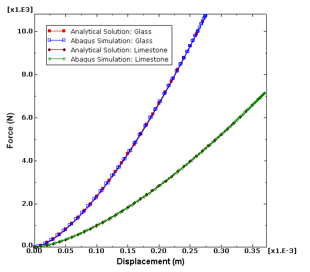
The elastic contact force is plotted against penetration (see Figure 1) for the two materials and for the analytical results. The maximum contact force, the maximum penetration, and the duration of contact are compared with the analytical results (see Chung, 2011), as shown in Table 5.

Table 5. Normal collision of two spheres.
Property	Glass		Limestone
Property	Abaqus	Analytical	Abaqus	Analytical
Contact duration (μs)	40.85	40.34	54.65	54.20
Maximum penetration (μm)	274.87	274.11	369.06	368.30
Maximum contact force (N)	10741.3	10696.9	7130.2	7108.1

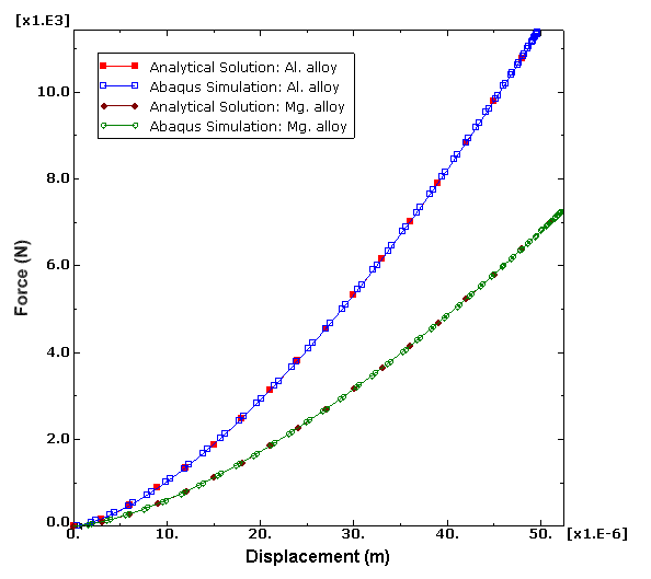
Test 2

The elastic contact force is plotted against penetration (see Figure 2) for the two materials and for the analytical results. The maximum contact force, the maximum penetration, and the duration of contact are compared with the analytical results (see Chung, 2011), as shown in Table 6.

Table 6. Normal collision of a sphere with a rigid plane.
Property	Aluminum alloy		Magnesium alloy
Property	Abaqus	Analytical	Abaqus	Analytical
Contact duration (μs)	732	731.59	767	766.99
Maximum penetration (μm)	49.71	49.72	52.12	52.12
Maximum contact force (N)	11369.4	11370.8	7232.1	7232.0

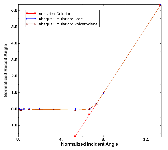
Test 3

The normalized incident angle, the normalized recoil angle, and the normalized postcollision angular speed for the sphere are calculated for each simulation. The normalized incident angle is the ratio of the precollision relative tangential velocity of the contact point of the spheres to the precollision relative normal velocity of the center of the spheres scaled by the friction coefficient. The normalized postcollision angular speed is the ratio of the postcollision angular speed scaled by the radius of the sphere to the postcollision normal velocity of the sphere. Figure 3 shows a plot of the normalized recoil angle versus the normalized incident angle compared with the analytical results. The normalized recoil angle is the ratio of the postcollision relative tangential velocity of the contact point of the spheres to the postcollision relative normal velocity of the center of the spheres scaled by the friction coefficient. Figure 4 shows a plot of the normalized postcollision angular speed versus the normalized incident angle compared with the analytical results. The plots in Figure 3 and Figure 4 show that sticking persists until the initial tangential velocity reaches a threshold value, beyond which slipping occurs during the collision.

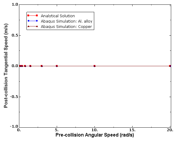
Test 4

Figure 5 shows a plot of the calculated postcollision tangential speed of the contact point versus the initial angular speed of the sphere compared with the analytical results. In Figure 6 the postcollision angular speed is plotted against the initial angular speed of the sphere along with the analytical results. Since the angular speed is the same for both the spheres with opposite direction of spin, no relative slip occurs during the collision; hence, the postcollision tangential velocity is absent. The comparison between the initial and the final angular speeds shows that there is no energy dissipation due to friction in this model because relative slip is absent.

Test 5

The tangent of the incident and the recoil angles are evaluated for each of the simulations. The recoil angle is the ratio of the relative tangential velocity of the contact point of the spheres to the relative normal velocity of the center of the spheres after the collision. The incident angle is the same quantity evaluated before the collision. Figure 7 shows a plot of the tangent of the recoil angle against that of the incident angle. As in test 3, below a threshold angular velocity, the smaller sphere sticks to the bigger sphere. Beyond this threshold value, it slips during the collision.

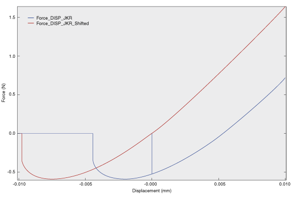
Test 6

The blue curve in Figure 8 shows the force-displacement response. The analytical value of the pull-off force is −0.589 N. The analytical value of the separation distance is −0.0044174 mm. Both of these values agree with the numerical results obatined from Abaqus/Explicit.

Test 7

The red curve in Figure 8 shows the force-displacement response. The analytical value of the pull-off force is −0.589 N. This is the same value as for the unshifted JKR adhesion model. The analytical value of the separation distance is −0.0097687 mm. Both of these values agree with the numerical results obtained from Abaqus/Explicit.

Input files

normal_identical_part_part.inp: Test 1: elastic head-on collision of two identical spheres.
normal_part_face.inp: Test 2: elastic normal impact of a sphere with a rigid plane.
oblique_part_face.inp: Test 3: oblique impact of a sphere with a rigid plane at a constant normal velocity and an incident angle.
normal_oppspin_identical_part_part.inp: Test 4: head-on collision of two identical spheres at the same translational speed, but with equal and opposite angular speed.
normal_spin_part_part.inp: Test 5: head-on collision of two different spheres with different translational and angular velocities.
part_part_jkr_jkrshift.inp: Test 6 and 7: normal contact between two spheres with JKR adhesion and shifted JKR adhesion models, respectively.
normal_identical_part_part_autodt.inp: Elastic head-on collision of two identical spheres using automatic time incrementation.
normal_part_face_autodt.inp: Elastic normal impact of a sphere with a rigid plane using automatic time incrementation.
oblique_part_face_autodt.inp: Oblique impact of a sphere with a rigid plane at a constant normal velocity and an incident angle using automatic time incrementation.
normal_oppspin_identical_part_part_autodt.inp: Head-on collision of two identical spheres at the same translational speed, but with equal and opposite angular speed using automatic time incrementation.
normal_spin_part_part_autodt.inp: Head-on collision of two different spheres with different translational and angular velocities using automatic time incrementation.
part_part_jkr_jkrshift_autodt.inp: Normal contact between two spheres with JKR adhesion and shifted JKR adhesion models, respectively, using automatic time incrementation.

References

Chung, Y. C., and J. Y. Ooi, “Benchmark Tests for Verifying Discrete Element Modelling Codes at Particle Impact Level,” Granular Matter, vol. 13, pp. 643–656, 2011.

Figures