Distributing coupling elements

This problem contains basic test cases for one or more Abaqus elements and features.

This page discusses:

Elements tested
Problem description
Reference solution
Results and discussion
Input files

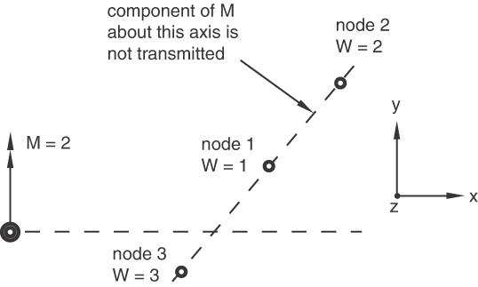
ProductsAbaqus/Standard

Elements tested

DCOUP2D

DCOUP3D

Problem description

The initial starting geometry for each test is shown in Figure 1. In the linear tests each coupling node is connected by a spring to ground (SPRING1) in each direction. In the geometrically nonlinear tests each coupling node is connected by a dashpot to ground (DASHPOT1) in each direction, and an axial spring element (SPRINGA) connects each pair of coupling nodes.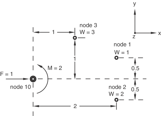

Distributing coupling elements connect a single reference node that has translational and rotational degrees of freedom to a collection of coupling nodes that have only translational degrees of freedom. Thus, when the coupling nodes are colinear, a situation can arise where the moments applied to the reference node are not transmitted by the element. This condition is relevant only for the three-dimensional version of the element. The third problem in this section tests the behavior of the element in this pathological situation.

Linear behavior

Properties:

The spring stiffnesses are 100, 200, and 300 for degrees of freedom 1, 2, and 3, respectively, for the springs connected to all coupling nodes. The mass of the distributing coupling is 10. The weight factors are 1, 2, and 3 for nodes 1, 2, and 3, respectively.

Loading:

Step 1: The force at node 10 is 1.0 in the x-direction. The moment at node 10 is 2.0 about the z-axis.

Step 2: (DCOUP3D only) The force at node 10 is 1.0 in the y-direction. The moment at node 10 is 2.0 about the x-axis.

Step 3: (DCOUP3D only) The force at node 10 is 1.0 in the z-direction. The moment at node 10 is 2.0 about the y-axis.

Step 4: Frequency extraction. (Step 2 for DCOUP2D)

Step 5: Transient modal dynamic step with a load, $F_{x} = $ 1.0 $\sin 2 π t$ , applied to node 10. (Step 3 for DCOUP2D)

Step 6: Mode-based steady-state dynamic step with a load, $F_{x} = $ 1.0, applied to node 10. (Step 4 for DCOUP2D)

Nonlinear behavior

Properties:

The dashpot damping coefficients are 100, 200, and 300 for degrees of freedom 1, 2, and 3, respectively, for the dashpots connected to all coupling nodes. The axial springs connecting the coupling nodes each have a spring constant of 1.0 × 10⁸. The mass of the distributing coupling is 10.

Prescribed reference node motion:

Step 1: Total rotation of $2 π$ about the z-axis. Translation $x = \sin 2 π t$ .

Step 2: (DCOUP3D only) Total rotation of $2 π$ about the y-axis. Translation $z = \sin 2 π t$ .

Step 3: (DCOUP3D only) Total rotation of $2 π$ about the x-axis. Translation $y = \sin 2 π t$ .

Step 4: Direct-integration dynamic step with a total rotation of $2 π$ about the x-axis. Translation $x = \sin 2 π t$ . (Step 2 for DCOUP2D)

Behavior with a colinear arrangement

Properties:

The spring stiffnesses are 100, 200, and 300 for degrees of freedom 1, 2, and 3, respectively, for the springs connected to all coupling nodes. The total mass of the model is 10; and mass elements are defined at nodes 1, 2, and 3.

Loading:

Step 1: The moment at node 10 is 2.0 about the z-axis.

Step 2: The moment at node 10 is 2.0 about the x-axis.

Step 3: The moment at node 10 is 2.0 about the y-axis.

Step 4: The moment at node 10 has a magnitude of 2.0 and is parallel to the coupling node colinear axis.

Step 5: Frequency extraction.

Reference solution

In all tests the load distribution among coupling nodes adheres to the relation

F^{n} = {\hat{w}}^{n} (F^{R} + T^{- 1} (M^{R} + r^{R} \times F^{R}) \times r^{n}),

where $F^{n}$ is the force distribution at the coupling nodes, $F^{R}$ and $M^{R}$ are the force and moment at the reference node, ${\hat{w}}^{n}$ are the normalized version of the weight factors specified with distributing coupling constraints, $T$ is the coupling node arrangement inertia tensor, and $r^{R}$ and $r^{n}$ are the positions of the reference and coupling nodes relative to the coupling node arrangement centroid, respectively. See Distributing coupling constraints for a more detailed description of this load distribution.

Results and discussion

The results for each problem are discussed below.

Linear behavior

Table 1. Displacements at node 10.
Step	$u_{1}$	$u_{2}$	$u_{3}$
1	6.67 × 10⁻³	−1.67 × 10⁻²	0.0
2	−2.06 × 10⁻³	1.35 × 10⁻²	−2.67 × 10⁻²
3	0.0	0.0	8.50 × 10⁻²

Table 2. Rotations at node 10.
Step	$ϕ_{1}$	$ϕ_{2}$	$ϕ_{3}$
1	0.0	0.0	1.05 × 10⁻²
2	1.33 × 10⁻²	−1.33 × 10⁻²	−7.33 × 10⁻³
3	−2.67 × 10⁻²	4.50 × 10⁻²	0.0

Table 3. Displacements at node 1.
Step	$u_{1}$	$u_{2}$	$u_{3}$
1	1.19 × 10⁻³	1.44 × 10⁻³	0.0
2	2.97 × 10⁻⁴	−5.78 × 10⁻⁵	6.67 × 10⁻³
3	0.0	0.0	−1.83 × 10⁻²

Table 4. NFORC output at node 2.
Step	NFORC1	NFORC2	NFORC3
1	1.39	0.574	0.0
2	−0.653	−2.31 × 10⁻²	−2.00
3	0.0	0.0	2.50

Table 5. Mode shape displacement components at node 10.
Mode	Eigenvalue	$u_{1}$	$u_{2}$
1	20.0	0.327	0.624
2	30.0	0.515	−0.653
3	40.0	−0.144	1.0

Table 6. Mode shape rotation components at node 10.
Mode	Eigenvalue	$ϕ_{3}$
1	20.0	−0.416
2	30.0	0.436
3	40.0	−0.345

Nonlinear behavior

All results correspond to the increment when the rotation is 3 $π /$ 4.

Table 7. Displacements at node 1.
Step	$u_{1}$	$u_{2}$	$u_{3}$
1	−3.06	0.561	0.0
2	−3.41	−2.22 × 10⁻⁴	−0.706
3	9.30410 × 10⁻⁵	−0.1451	0.353
4	−3.06	0.561	5.51 × 10⁻⁵

Table 8. NFORC output at node 1.
Step	NFORC1	NFORC2	NFORC3
1	−679	−1080	0.0
2	−1090	−47.7	1120
3	−8.46	−1190	−757
4	−623	−1270	4.44 × 10⁻²

Table 9. Displacements at node 2.
Step	$u_{1}$	$u_{2}$	$u_{3}$
1	−2.35	2.27	0.0
2	−3.41	−2.22 × 10⁻⁴	−0.706
3	−9.31 × 10⁻⁵	1.56	−0.354
4	−2.35	2.27	6.87 × 10⁻⁵

Table 10. NFORC output at node 2.
Step	NFORC1	NFORC2	NFORC3
1	−2090	−1420	0.0
2	−935	−95.4	1270
3	186	−313	563
4	−1970	−1820	1.83 × 10⁻²

Behavior with a colinear arrangement

Table 11. Displacements at node 10.
Step	$u_{1}$	$u_{2}$	$u_{3}$
1	1.59 × 10⁻³	−7.69 × 10⁻³	0.0
2	0.0	0.0	−2.06 × 10⁻³
3	0.0	0.0	2.06 × 10⁻³
4	0.0	0.0	0.0

Table 12. Rotations at node 10.
Step	$ϕ_{1}$	$ϕ_{2}$	$ϕ_{3}$
1	0.0	0.0	3.76 × 10⁻³
2	8.36 × 10⁻⁴	−8.36 × 10⁻⁴	0.0
3	−8.36 × 10⁻⁴	8.36 × 10⁻⁴	0.0
4	0.0	0.0	0.0

Table 13. Displacements at node 1.
Step	$u_{1}$	$u_{2}$	$u_{3}$
1	3.45 × 10⁻⁴	−1.72 × 10⁻⁴	0.0
2	0.0	0.0	−1.15 × 10⁻⁴
3	0.0	0.0	1.15 × 10⁻⁴
4	0.0	0.0	0.0

Table 14. NFORC output at node 2.
Step	NFORC1	NFORC2	NFORC3
1	0.483	−0.483	0.0
2	0.0	0.0	−0.483
3	0.0	0.0	0.483
4	0.0	0.0	0.0

Table 15. Mode shape displacement components at node 10.
Mode	Eigenvalue	$u_{1}$	$u_{2}$
1	20.0	0.327	0.560
2	30.0	0.494	−0.523
3	40.0	0.172	−6.03 × 10⁻²

Table 16. Mode shape rotation components at node 10.
Mode	Eigenvalue	$ϕ_{3}$
1	20.0	−0.259
2	30.0	0.241
3	40.0	0.259

Input files

exdc2lx1.inp: Linear behavior of DCOUP2D elements with LOAD CASE.
exdc3lx1.inp: Linear behavior of DCOUP3D elements.
exdc2nx1.inp: Geometrically nonlinear behavior of DCOUP2D elements.
exdc3nx1.inp: Geometrically nonlinear behavior of DCOUP3D elements.
exdc3cx1.inp: Test of DCOUP3D elements with colinear coupling nodes.