Connected fluid cavities
Elements tested
FLINK
F2D2
Problem description
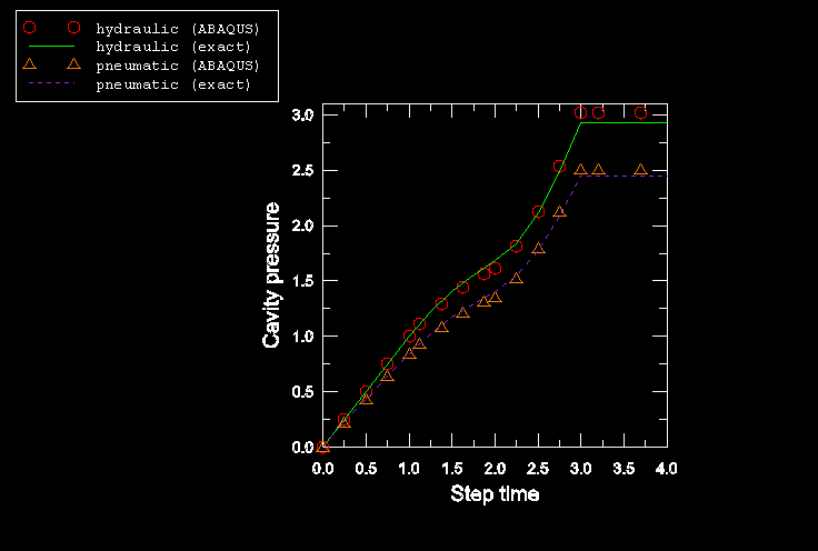
A fluid link element is created when the fluid exchange capability is used to transfer fluid between two vessels filled with incompressible fluid, as shown in Figure 1. One of the vessels is subjected to internal pressure by applying a load F. The other vessel is always maintained at zero pressure. The difference in pressures between the two vessels causes fluid to be transferred. Two analyses are performed to verify the fluid transfer rate between the two vessels by specifying the bulk viscosity and the mass flow rate as a function of pressure difference and temperature.
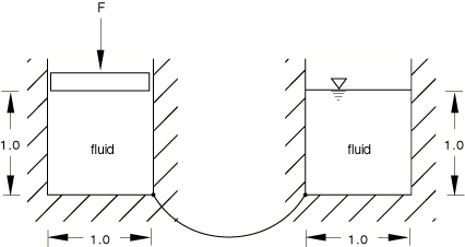
Each vessel is modeled using a two-dimensional fluid block that measures 1 × 1 with unit thickness, as shown in Figure 2. Nodes 1 and 11 are the cavity reference nodes for the two fluid cavities. The downward force on the first fluid cavity is applied as a concentrated load to node 4 in the y-direction. Nodes 3 and 4 are constrained to displace equally in the y-direction. Nodes 13 and 14 are also constrained to displace equally in the y-direction. Finally, grounded springs of very small stiffness acting in the y-direction are attached to nodes 4 and 14 to preclude solver problems in the solution.

Material:
Fluid: incompressible, density = 10.0 (arbitrary).
Fluid link:
| Specifying the bulk viscosity | |||
| Field variable | |||
| 10 | 0.0 | 10 | 1.0 |
| 1.0 | 0.0 | 100 | 1.0 |
| 10 | 0.001 | 10 | 2.0 |
| 1.0 | 0.001 | 100 | 2.0 |
The data used when specifying the mass flow rate as a function of pressure difference and temperature were computed using the implicit functional relationship between q and discussed in Fluid Exchange Definition, and the values of and in the above table. To capture the nonlinear relationship between q and accurately, 33 values of q were included in the data lines option for various combinations of and the one field variable.
Loading:
The concentrated force of 100 units is applied instantaneously over all static steps. In the first step the temperature and the field variable are held fixed at 10 and 1, respectively, for a time period of 0.20. In the second step the temperature is ramped from 10 to 100 for a time period of 0.01, while the field variable remains fixed at 1. The third step is a dummy perturbation step. This step is included to verify that an intermittent perturbation step has no effect on the subsequent general step. In the fourth step the temperature is held fixed at 100, with the field variable instantaneously changed to 2 for a time period of 0.01. Results are reported at the end of each general step.
Reference solution
Since the fluid is incompressible, the total fluid volume should be maintained; i.e., CVOL=2.0. The pressure in the first cavity should always be 100. Because of the presence of grounded springs of very small stiffness, the pressure in the second cavity is not zero.
Results and discussion
The results for the analyses compare quite well with one another. The agreement between the two models could be further improved by refining the tabular data for the mass flow rate model to better represent the nonlinear relationship between q and as defined by the bulk viscosity model.
| Specifying the bulk viscosity | ||||
|---|---|---|---|---|
| Step | PCAV | CVOL | PCAV | CVOL |
| 1 | 100.0 | 0.800 | 2.00E−7 | 1.20 |
| 2 | 100.0 | 0.778 | 2.22E−7 | 1.22 |
| 4 | 100.0 | 0.683 | 3.17E−7 | 1.32 |
| Specifying the mass flow rate as a function of pressure difference and temperature | ||||
|---|---|---|---|---|
| Step | PCAV | CVOL | PCAV | CVOL |
| 1 | 100.0 | 0.800 | 2.00E−7 | 1.20 |
| 2 | 100.0 | 0.778 | 2.22E−7 | 1.22 |
| 4 | 100.0 | 0.683 | 3.18E−7 | 1.32 |
Input files
- efl2sfsp.inp
TYPE=BULK VISCOSITY.
- efl2stsp.inp
TYPE=MASS RATE LEAKAGE.