Tire deflation with adaptive meshing
Elements tested
- ACAX4
- ACAX8
- AC3D8
- AC3D20
Features tested
Adaptive meshing, user-specified normal definition at a node, symmetric model generation, and symmetric boundary conditions.
Problem description
Model:
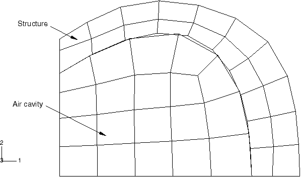
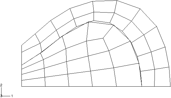
A simple tire filled with air is analyzed, as shown in Figure 1. We model half of the cross-section. A negative pressure is applied to the inside of the structure, causing a significant decrease in the volume of the acoustic domain. We apply adaptive mesh smoothing after each converged structural load increment to compute a new acoustic mesh. We extract the eigenvalues of the coupled system after the preloading is applied. These eigenvalues are compared with the eigenvalues obtained in an independent analysis in which no adaptive mesh smoothing is performed. In this reference analysis both the acoustic mesh and structural mesh are defined in the displaced configuration. We apply an initial stress state that is in equilibrium with the pressure load so that no deformation takes place. The displaced configuration for the acoustic mesh is extracted from the results file. The displaced configuration for the structural mesh as well as the associated solution state that serves as the initial condition are obtained when the reference configuration is updated.
We also perform the same analysis using a three-dimensional model. We generate the model using symmetric model generation.
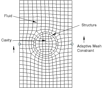
This example tests a number of adaptive mesh smoothing features. The adaptive mesh domain contains different node types, including interior nodes, corner nodes, surface nodes, nodes tied to the structure, as well as acoustic nodes that are connected using a tie constraint. The different updating rules associated with each of these node types are tested. In addition, application of the pressure load causes the volume of the acoustic elements to become negative. This, in turn, causes geometric feature changes (a corner develops) along the vertical surface. To avoid the development of corners, we transfer the structural displacement over a series of sub-increments to the acoustic domain. Adaptive meshing is applied after each sub-increment. The development of the corner can also be avoided by applying adaptive mesh controls. Both features are tested. Finally, the normal direction on the surface between the acoustic domain and structural domain is not computed correctly by Abaqus on a symmetry plane. The correct normal can be defined by using an alternative normal definition of contact surfaces or by applying symmetry boundary conditions. This example verifies that both these features are applied correctly during adaptive mesh smoothing.
Results and discussion
Figure 2 shows the displaced configuration. The eigenvalues agree closely with the reference solution, indicating that the geometry of the acoustic domain is updated correctly. The response of the system to harmonic excitation is obtained using mode-based, direct-solution, and subspace-based steady-state dynamic analysis. The results agree well between the three analysis types.
Input files
- am_tireair_acax4.inp
-
Axisymmetric tire-air model with ACAX4 elements and symmetric boundary conditions.
- am_tireair_acax4_normal.inp
-
Axisymmetric tire-air model with ACAX4 elements and NORMAL.
- am_tireair_acax4_tie.inp
-
Axisymmetric model with two acoustic regions connected using TIE.
- am_tire_acax4.inp
-
Axisymmetric tire problem used as base state for the reference solution.
- am_tireair_acax4_ver.inp
-
Axisymmetric tire-air problem used as a reference solution.
- am_tireair_ac3d8.inp
-
Three-dimensional tire-air interaction with AC3D8 elements.
- am_tire_ac3d8.inp
-
Three-dimensional tire problem used as base state for obtaining the reference solution.
- am_tireair_ac3d8_ver.inp
-
Reference solution for three-dimensional model.
- am_tireair_acax8.inp
-
Axisymmetric tire-air interaction with ACAX8 elements.
- am_tire_acax8.inp
-
Axisymmetric tire problem used as base state for reference solution.
- am_tireair_acax8_ver.inp
-
Axisymmetric model used as reference solution for second-order elements.
- am_tireair_ac3d20.inp
-
Three-dimensional model with AC3D20 elements.
Figures