Uniaxial tension with initial stress, T3D2 elements.
Drucker-Prager plasticity with linear elasticity
Elements tested
C3D8
C3D8R
CAX4
CPE4
CPS4
Problem description
Material:
Elasticity
Young's modulus, E =
300.0E3
Poisson's ratio,
= 0.3
Plasticity
Angle of friction,
= 40.0
Dilation angle,
= 40.0
Third invariant ratio, K = 0.78 (when included;
otherwise, 1.0)
Hardening curve:
Yield stress
Plastic strain
6.0E3
0.000000
9.0E3
0.020000
11.0E3
0.063333
12.0E3
0.110000
12.0E3
1.000000
(The units are not important.)
The hyperbolic and exponent forms of the yield criteria are verified by
using parameters that reduce them into equivalent linear forms. Reducing the
hyperbolic yield function into a linear form requires that
.
Reducing the exponent yield function into a linear form requires that
b = 1.0 and that a =
()−1.
Results and discussion
Most tests in this section are set up as cases of the homogeneous deformation of a single element
of unit dimensions. Consequently, the results are identical for all integration points
within the element. To test certain conditions, however, it is necessary to set up
inhomogeneous deformation problems. In each case, the constitutive path is integrated with
20 increments of fixed size.
Explicit dynamic continuation of sx_s_druckerprager.inp with both the
reference configuration and the state imported, C3D8R elements, uniaxial tension.
Import into
Abaqus/Standard
from sx_x_druckerprager_y_y.inp with both the reference configuration and the
state imported, C3D8R elements, uniaxial tension.
Import into
Abaqus/Standard
from sx_x_druckerprager_n_n.inp without importing the state or the reference
configuration, C3D8R elements, uniaxial tension.
Drucker-Prager plasticity with porous elasticity
Elements tested
CAX4
Problem description
Material:
Elasticity
Logarithmic bulk modulus,
= 1.49
Poisson's ratio,
= 0.1
Plasticity
Angle of friction,
= 10.0
Dilation angle,
= 10.0
Hardening curve:
Yield stress
Plastic strain
100.0
0.0
500.0
0.5
Initial
conditions
Initial void ratio,
= 4.1
The hyperbolic and exponent forms of the yield criteria are verified by
using parameters that reduce them into equivalent linear forms. Reducing the
hyperbolic yield function into a linear form requires that
.
Reducing the exponent yield function into a linear form requires that
b = 1.0 and that a =
()−1.
(The units are not important.)
Results and discussion
The tests in this section are set up as cases of homogeneous deformation of a single element of
unit dimensions. Consequently, the results are identical for all integration points within
the element. In each case, the constitutive path is integrated with 20 increments of fixed
size.
In the tests described in this section, the following data for linear
elasticity, cap plasticity I, cap hardening I, and K = 1.0
are used unless otherwise specified. With this data, the elastic shear modulus
is 5000.0 and the bulk modulus is 10000.0. First yield in pure shear occurs at S12 = 100.0, first yield in pure hydrostatic compression occurs at PRESS = 270.0, first yield in pure hydrostatic tension occurs at PRESS = 300.0, and first yield with PRESS =
occurs at PRESS = 120.0 and S12 = 125.0. C3D8 elements are used unless otherwise specified.
Linear elasticity (used in nearly
all tests)
Young's modulus, E = 12857.1429
Poisson's ratio,
= 0.28571429 (= 1/7)
Cap plasticity I
(used in nearly all tests)
Cohesion, d = 173.20508 (= 100)
Slope of Drucker-Prager failure surface,
= 30.0
Cap ellipticity, R = 0.61858957
Initial volumetric plastic strain,
= 0.027
Transition parameter,
= 0.69258232
Third invariant factor, K = 1.0 or 0.8, depending on
the test.
Cap hardening I
(used in nearly all tests)
Position of the yield surface in pure hydrostatic compression,
Volumetric compressive plastic strain,
213.0
0.00
222.0
0.01
242.0
0.02
282.0
0.03
362.0
0.04
522.0
0.05
842.0
0.06
1482.0
0.07
2762.0
0.08
Cap
plasticity II
d = 0.2286E6
= 85.0
R = 0.0875
= 1.22
= 0.07877
K = 1.0
Cap hardening
II
Position of the yield surface in pure hydrostatic compression,
Volumetric compressive plastic strain,
0.03E6
0.0
0.20E6
1.22
2.00E6
2.44
2.00E7
3.66
Porous
elasticity I
Logarithmic bulk modulus,
= 20.0
Poisson's ratio,
= 0.28571429
Tensile strength limit,
= 1.0E5
Porous
elasticity II
= 0.09
= 0.0
= 0.02E6
Initial
conditions
Initial void ratio,
= 1.0
Results and discussion
The results agree well with exact analytical or approximate solutions.
Uniaxial compressive strain (odometer) test; CPE4 element; load control; with temperature and field variable
dependence of the
CAP PLASTICITY and
CAP HARDENING data.
The temperatures and field variables are specified to give
CAP PLASTICITY and
CAP HARDENING data exactly the same as cap plasticity I and cap
hardening I data.
Uniaxial compressive strain (odometer) test; load control; the nonlinear
analysis is split into two steps, each of which is preceded by a linear
perturbation step.
The results of the nonlinear steps should correspond to those of
mca0003bus.inp.
The results of the two linear perturbation steps (STATIC) should be identical because small displacements are
assumed and the elasticity is linear.
Linear perturbation with
LOAD CASE and hydrostatic compression, C3D8 elements.
Clay plasticity with linear elasticity
Elements tested
C3D8
C3D8R
CAX4R
CAX8R
CPE4R
Problem description
Material 1
Elasticity
The Young's modulus used in each test is given in the input file
description. The modulus of each test is based on the average elastic stiffness
of the equivalent test with porous elasticity at increments 10 and 20. A direct
comparison with the results documented in
Drucker-Prager plasticity with linear elasticity
is, therefore, possible.
Poisson's ratio,
= 0.3
Plasticity
Critical state slope, M = 1.0
Initial volumetric plastic strain,
= 0.4
Cap parameter,
= 0.5 (when included; otherwise, 1.0)
Third invariant ratio, K = 0.78 (when included;
otherwise, 1.0)
The exponential hardening curve used in
Drucker-Prager plasticity with linear elasticity
is entered in tabulated form with an initial volumetric plastic strain that
corresponds to a yield surface size of either
= 58.3 or
= 130.9.
(The units are not important.)
Material 2
Elasticity
Young's modulus,
= 18820
Poisson's ratio,
= 0.3
Plasticity
Critical state slope, M = 1.0
Initial volumetric plastic strain,
= 0.0
Cap parameter,
= 1.0
Third invariant ratio, K = 1.0
Tabulated curves are used for defining the compressive and tensile
hardening.
Softening
regularization
= 0.8
= 2.0
= 2.5
(The units are not important.)
Material 3
Elasticity
Young's modulus,
= 18820
Poisson's ratio,
= 0.3
Plasticity
Critical state slope, M = 1.0
Initial volumetric plastic strain,
= 0.0
Cap parameter,
= 1.0
Third invariant ratio, K = 1.0
Tabulated curves are used for defining the compressive and tensile
hardening.
Softening
regularization
= 0.5
= 1.0
= 2.5
(The units are not important.)
Material 4 [Crook et al. (2002)]
Elasticity
Engineering constants
200000.0
342000.0
342000.0
0.32
0.32
0.32
89900.0
89900.0
129545.5
Plasticity
Critical state slope, M = 1.0
Initial volumetric plastic strain,
= 0.0
Cap parameter,
= 1.0
Third invariant ratio, K = 1.0
Tabulated curves are used for defining the compressive and tensile
hardening.
Crook, A.
J.
L., J.
G. Yu, and S.
M. Willson, “Development of an Orthotropic 3D
Elastoplastic Material Model for Shale,”
SPE/ISRM Paper SPE 78238,
2002.
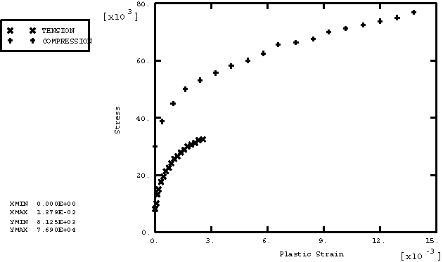
Hardening curves: The hardening curves in tension and compression are
illustrated in
Figure 1.
Thermal
properties
Specific heat,
= 47.52
Density,
= 439.92
Conductivity, k = 9.4
Coefficient of expansion,
= 11.0E−6
Figure 1. Stress versus plastic strain under uniaxial tension and uniaxial
compression.
(The units are not important.)
Results and discussion
Most tests in this section are set up as cases of the homogeneous
deformation of a single element of unit dimensions. Consequently, the results
are identical for all integration points within the element.