Impedance boundary conditions

The impedance boundary conditions are tested in this verification set. The model consists of a column of fluid 10 meters high with a cross-sectional area of 1 m. The first-order element models consist of 20 acoustic elements: 20 high and one in the cross-section. The second-order element models consist of 10 elements along the height direction.

One end of the column has a surface impedance imposed on it that is set equal to the characteristic impedance of the fluid column, $Z={\rho }_{f}c$, where ${\rho }_f$ is the density of the fluid and $c=\sqrt{K_f/{\rho }_f}$ is the speed of sound in the fluid. To simulate a nonreflecting boundary condition, $1/c_1=1/Z$ and $1/k_1=$ 0 are set with an impedance boundary condition. The material used in these tests is air with the following properties: density, ${\rho }_f=$ 1.293 kg/m³; bulk modulus, $K_f=$ 1.42176 × 10⁵ N/m²; and $1/c_1=1/Z=$ 2.3323 × 10⁻³ m²s/kg.

The other end of the column is excited by a harmonic pressure impulse of magnitude 1.0 N/m². A steady-state dynamic analysis is performed in Abaqus/Standard over a range of frequencies from 0 to 100 Hz. Transient simulations are also performed in Abaqus/Explicit using an excitation frequency of 100 Hz. Different excitation frequencies can be tested by changing the parameters defined in the input files. The solution should represent a steady-state unattenuated wave moving in the positive y-direction. No resonating frequencies should result; the maximum pressure throughout the column should consistently remain at a magnitude of 1.0 N/m², and the phase should drop by 2$\pi$ radians over the distance of a wavelength, $\lambda =c/f$, where f is the excitation frequency in cycles per time.

These tests model a sound source at $x=$ 0 m in a tube with significant volumetric drag (air properties with $\gamma =$ 1400 Ns/m⁴) and a nonreflective end condition at $x=$ 0.5 m at a frequency of 100 Hz. The complex density of the acoustic medium is specified in a second part in these analyses. In each model the inward acceleration of the sound source is specified as the complex value $a=\omega i$, giving an inward velocity of 1 m/s. (The inward acceleration on a face is distributed to the nodes of the face as concentrated loads representing inward volume accelerations in the same way as pressure on a face would be distributed to the nodes of the face as concentrated loads representing nodal forces.) Because of the large drag, for good results at this frequency the constants $1/c_1$ and $1/k_1$ must both be nonzero and must be based on the complex impedance of the medium.

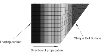
These tests model one-dimensional propagation of sound in situations where the acoustic waves exit the acoustic domain through oblique boundaries. Various elementary geometric shapes are tested. In all models sinusoidal acoustic pressure boundary conditions are applied on one face of the acoustic domain, resulting in one-dimensional acoustic wave propagation in the model. The models are created so as to force the acoustic waves to exit from the model via surfaces that possess either continuously varying normals or normals that are not oriented in the same direction as the propagation of the waves. On the exit surface an impedance condition is used. The objective in all the models tested is to ensure that the problem remains one-dimensional and that there is no reflection of the acoustic waves back into the domain from the oblique boundary.

For the ASI element tests the physical problem is similar to the nonreflective boundary test. Here, however, there is no volumetric drag, and a portion of the length of the body of air in the tube is modeled with truss elements. These are given Young's modulus and density to match the bulk modulus, $K_f=$ 1.424 × 10⁵ N/m², and density, ${\rho }_f=$ 1.21 kg/m³, of air. The rest of the tube is modeled with acoustic elements that have the properties of air. Acoustic-structural coupling is set up between the structural region and the acoustic region using ASI elements, and a nonreflective end condition is applied.

This problem is analyzed for the one-dimensional case using ASI1 elements, for the two-dimensional case using ASI2 and ASI3 elements, for the axisymmetric case using ASI2A and ASI3A elements, and for the three-dimensional case using ASI4 and ASI8 elements. All the nodes in these models are constrained such that they have only the horizontal translation degree of freedom to simulate one-dimensional wave propagation.

These tests compare the behavior of acoustic infinite elements with and without impedance conditions defined on the semi-infinite sides. In all models the acoustic infinite elements are coupled directly to structural elements using steel material properties. The acoustic infinite elements use air properties and an impedance condition on one semi-infinite side with a tabular value corresponding to one-half the material impedance. In the steady-state dynamic analyses the frequency is varied from 1 to 200 Hz. In the transient dynamic analyses the elements are excited using a sinusoidal amplitude with an angular frequency of 5.