Analyzing Variable Dependencies for a Normal Simulation
You can work with variable dependencies for normal simulation.
For an example, see Analyzing Variable Dependencies for a Normal Simulation.
Analyzing Variable Dependencies for a Normal SimulationYou can work with variable dependencies for normal simulation. For an example, see Analyzing Variable Dependencies for a Normal Simulation. Analyzing Variable Dependencies for a Failed Initialization of a SimulationYou can analyze variable dependencies for a failed initialization of a simulation.
For more information on how to reach these options, see Setting up a Simulation. For more information about the dialog box alternatives, see Simulation Setup Dialog Box. For an example where the feature of analyzing variable dependencies can be used, see Analyzing Variable Dependencies for a Normal Simulation. Notes:
Analyzing Equation IncidenceYou can work with equation incidence to explore the structure of a translated model. You can also use the equation incidence as a tool for debugging a simulation failure. In this section, you explore the structure of a translated model example using the equation incidence graph. To display and simulate the model example ControlledTanks1, do the following:
The example consists of two tanks, three valves, and a state machine controlling the valves. During simulation, valve1 opens to fill up tank1 with water from the reservoir. When tank1 is full, its content is drained into tank2, making a pause when the former tank is almost empty. Finally, tank2 is emptied and the cycle repeats. To run the example to see how it works, replay the animation. For more information, see Replaying an Animation. To display the equation incidence graph for the model, do the following:
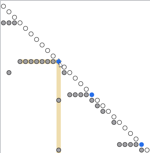
The Equation Incidence window contains three panes. The middle pane displays the dependency graph as a sorted Block Lower Triangular (BLT) form of equation blocks, graphically indicated by nodes. The graph´s diagonal contains either scalars, which are represented as white nodes, or systems of equations, marked by colored nodes. The full color coding of the nodes of the diagonal is:
In there are three blue nodes indicating that there are three systems with mixed continuous and discrete equations. Notes:
 In the current model, this example, the upper pane (not displayed in the figure), you get information of what kind of equation block you have selected. In the lower pane (not displayed in the figure below), you get a list of all the variables the equation block solves for. This includes iteration variables, torn variables, as well as discrete variables. For this example, you can see from the list that this system solves for the flow and pressures around valve2, between the two tanks. The gray off-diagonal nodes represent dependencies. If you click a gray node, you see the corresponding dependency equation in the upper pane. The gray nodes to the left of the blue node, on the same row, represent variables that need to be computed before the first system can be solved. That is, they represent upstream dependencies for that system. The gray nodes below the blue node, in the same column, show where variables from the first system are used in subsequent computations. That is, they represent downstream dependencies for that system. Note:
For upstream dependencies, the difference compared to the plot
dependencies feature is that an equation incidence node can represent several
variables as part of the same upstream dependency.
An important use of the equation incidence graph is to investigate if the systems are independent of each other. The first system calculated is by definition independent. To investigate if the second system is independent of the first system, look at the figure above. You can see that the first gray node in the column appears after the line of the second system, meaning that this dependence is not relevant until after the second system has been computed. That is, the second system is independent of the first system. To investigate if the third system is independent of the second system, select the
second system as below: In a similar way, you can prove that the third system is independent of the first system. Note:
To be able to easier slide along the diagonal, you can activate Rotate
the incidence matrix 45°. This is the default, but it is easier to
explain the indecence graph when this option is not activated.
| |||||||||||||||||||||