-
From the Scenario section of the action bar, click Simulation
Analysis
 . .
-
Click the Numeric Integration tab.
The Numeric Integration tab contains the
following columns:
- The state variable name.
- The number of times the variable limits the step size of the
numerical integrator. Counts greater than zero are
highlighted.
- The number of times the variable dominates the error, that is,
has an integration error larger than any other state variable.
Counts greater than zero are highlighted.
- The number of times the variable contributes to more than 10 %
of the integrator error.
Notes:
- You can click any column header to sort the lines in
descending or ascending order.
- The window can be minimized. It is then displayed with the
icon on the right side of the screen.
- If no information can be displayed, the Numeric
Integration tab is not displayed.
- To display the result for a variable in a plot, right-click the variable in the window and select Plot Error.
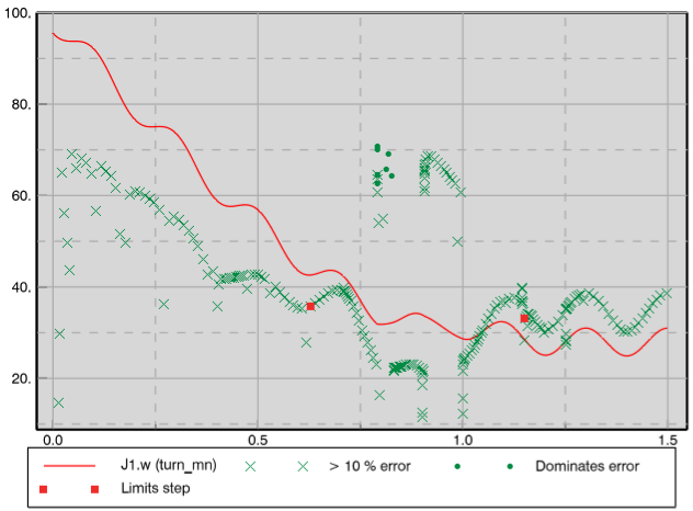
The following is the result: - In the plot that appears a marker is plotted at each time point where such an event occurs, and
the value on the vertical axis is the contribution to the
numeric error in percent. This plot gives a better understanding
of the variable´s effect on the numeric integrator at various
stages of the simulation.
To see an
example, right-click J1.w in the
window and select Plot Error. The
result is:

You can see that the variable
J1.w dominates the error around
t=0.8, but not at t=0.9-1.0 although the error is still
larger than 60 %. The variable J1.w
limits the step size near t=0.65 and T=1.15. - The variable that you selected is also highlighted in the Variable Browser.
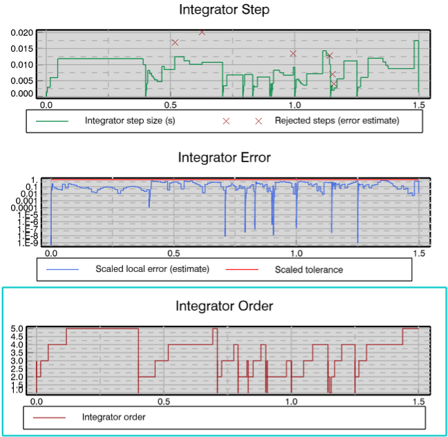
- To study the behavior of the numeric integrator, click Plot Integrator Step Size.
A plot appears, displaying the internal integrator step size, the scaled local error
estimate from the integrator, and the integration order. Notes:
- Rejected steps (and subsequent restart with smaller step)
are indicated with red cross.
- You can use the scaled local error estimate to, for example,
see if the integration step size is being limited by the
error estimate or something else, like frequent restarts
because of events.
.

|