You can use weight to view
the predefined metrics, drill-down, and analyze data.
To filter on structure, you can decide on which configuration the assessment is applied. Once
you select a configuration, the assessment roll-up starts. The rolled-up value versus the
objective value is displayed on the configured element.
You can display the multi-KPI dashboard in
Weight and Balance.
From the Compass, drag the Weight and Balanceapp from
the Compass to your dashboard.
Optional:
To verify the server status, click Check server status and select
Dispatcher, Orpheus Controller and
Orpheus Instance.
You can see blue indicators when the status is valid, or gray indicators when
it is not. A tooltip indicates what you should do or provides the index scan date.
Search for an element containing metric values in the 3DSearch and drag it onto Weight and Balance.
The weight, center of gravity, and inertia matrix metrics are displayed.
Note:
The label contour of the metrics is:
Gray (no contour) when no objective has been defined for this element.
Green when the objective is reached.
Yellow when the objective is in the minimum - maximum interval.
Red when the metric has an objective but no value, or when the objective is not
reached, or out of the minimum - maximum interval.
Optional:
Select a Configuration Filter.
If several configurations are available for this item, you can select one of them.
You can also compare different configurations.
Tip:
When your component has more than six configurations, a search box is
displayed and you can filter the list.
The web app
displays the consolidated metrics for this item. If you click the thumbnail, a tooltip
displays the metric values.
To display all the existing metrics, click All KPIs.
When a label is selected, the metric name is displayed at the
top of the window (Global Scoring > Weight).
Assess the Weight
You can see the detailed analytics of the weight.
Click the weight's metric label.
Compare the weight of the item and the defined targets.
The following information is displayed:
Weight: Mass of the item, with the fluid weight included when the item (a pipe) contains a fluid;
therefore, the mass of the item is called the wet weight. For more information, see Assess the Fluid Weight and the Dry Weight.
Objective: Value to reach for the selected element. There
is not any value nor assessment gauge when objectives have not been defined (see the
image below).
Tolerance: Statistical consolidation of tolerances on
children.
Confidence: Consolidation of the confidence percentage.
Budget: Sum of all budgets defined on every level of the
structure.
Tip:
Click More Details to visualize other
analytics such as Tolerance and Budget.
Assessment gauge chart: An assessment of a specific metric
regarding its objectives. A colored gauge replaces the image with the "No objectives
defined" information, when objectives have been specified. For more information, see
About the Assessment Gauge.
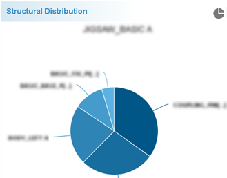
Structural Distribution: A pie chart to focus on the weight distribution for the selected element. For more
information, see Structural Distribution.
Weight Trend: A trend chart appears only if you added metrics
to the timeline before. You can select other attributes in the list. See Display the Timeline Chart.
To go back to the weight, center of gravity, and inertia matrix metrics' page, click Global
Scoring.
Assess the Fluid Weight and the Dry Weight
When a physical product includes pipes filled with liquid material, the fluidic
mass is computed. A separate secondary analytics provides the fluidic weight and the dry weight.
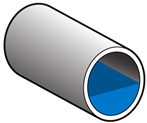
Pipe without fluid:
Pipe with fluid:
Before you begin: To perform this task,
To compute the wet weight of
the product, taking the LineID modification into account, open Weight Analysis.
From the 3DEXPERIENCE or the 3DDashboard, search for an element with pipes containing fluid in
the 3DSearch.
Do one of the following:
From the 3DEXPERIENCE, open the element and click Weight and Balance
from the Data Intelligence section of the action bar.
Or from the 3DDashboard, drag it onto the Weight and Balanceapp to compute the metrics.
Click the weight's metric label.
Notes:
The fluid mass affects the value of the weight metric. The total mass of the item is: the mass
of the structure, plus the fluid weight.
The value of the inertia matrix varies with the liquid weight.
The value of the center of gravity remains the same for leaf nodes as the fluid's
center of gravity is approximately the same as the pipe
structure's.
For intermediary nodes, the fluid weight impacts their center of gravity, as it is proportional to the wet weight of its leaf children.
To get the detailed analytics of weight metric as dry and fluid weight, click Analytics and select
Dry Weight, Wet Weight.
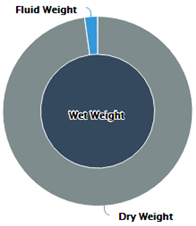
A pie chart with color codes displays the distribution of the dry (gray), fluid
(light blue) and wet (dark blue) weight: Dry weight, wet weight pie chart
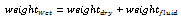
The wet weight is the sum of dry weight and fluid weight: . It is
indexed in the Cloud View.
To compare the business values of the weight metric with previous ones, select the Dry
Weight, Wet Weight Trend. For more information, see Add to the Timeline and Display the Timeline Chart.
A historical graph displays the previous dry and fluid weight analytics, saved during a timeline edition.
There is a legend for the metric values, the objectives and the dry and fluid weight trends, therefore, you can also compare the wet weight value with the predefined metric objectives.
To go back to the weight, center of gravity, and inertia matrix metrics' page, click Global
Scoring.
Structural Distribution
You can see the metric structural distribution in an assembly and drill-down to the
metric structure from an item.
You can display its consolidated metric information in a pie chart or multi-list view, and
customize it in the assessment apps only.
Click the label of the metric.
Select Structural Distribution to
get an assessment of an item from the assembly in a dedicated tab. You can display the
assessment in a pie chart view (default option) or in a multilist view:
Pie chart view:
By
default, the pie chart view is displayed.
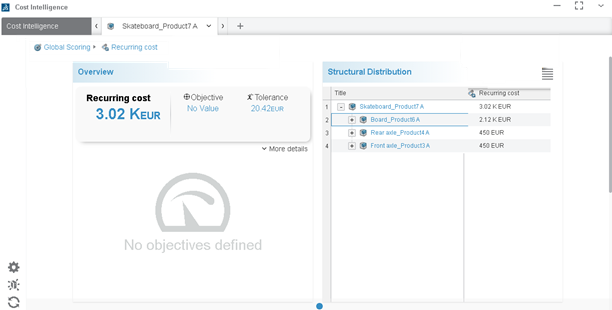
Multilist view (example of a Cost metric).
Note:
You can switch between the pie chart view and the multilist view by clicking
the button or
in
the right corner of the panel.
The multilist view is available for all the assessment apps and provides all the metrics in a single view along with its drill-down.
There are headers and subheaders for each metric based on the cockpit. You can
customize the display of the headers by selecting the following contextual
commands on the cells. For more information, see the next step.
The first column displays the title header of the item along with its revision
and its structure in a tree. The multilist view also displays data coming from different facets, for
example: Manufacturing, Operation etc. The data coming from the facet is one
level below the context item. A mask appears on the type icon: .
The second column displays the metric values along with the assessment icon
(only if the objective is set).
Assessment Icon
Assessment Detail
On Target
If the value and its objective are the same.
Over or Under
Target
If the value is outside target range of the objective.
Within Target
If the value is within the target range of the objective but is not
the targeted value. This case is specific to the objective within
range.
Here is an example of an assessment icon:
You obtain, for example, a consolidated metric information of a metric from its
Engineering or Manufacturing structure.
Note:
The drill-down is always one level.
Click an element either in the pie chart or in the dedicated tab and select a contextual command.
Command
Functionality
Open in a new tab
Launches the selected item in a separate tab of the assessment app.
Drill down into this element
Opens one level drill-down to reveal the child items and its metrics.
Select in 3D
Cross-highlights the selected item in the 3D Navigate app.
Note:
This command is only available when the assessment app has been paired with the 3D Navigate app.
Cancel selection and reveal
Removes the cross-highlighting after the Select in 3D command is
executed.
Note:
This command is only available when the assessment app has been paired with a 3D Navigate app.
To customize the multilist view columns, select the Column
Customization contextual command.
A panel is displayed containing two tabs:
Metric:
Displays the entire metrics specific to the cockpit in a numbered list. You can
select one or several metrics. Your selection is persistent for the given
widget. At least one metric should be selected, otherwise an error message
appears.
Metric Info:
Displays a selection list containing the Value,
Confidence, Tolerance,
Budget, Objective, and
Assessment parameters. The Value
option is selected by default and cannot be cleared. Your selection is also
persistent. You can reorder the Metric Info subheader in the multilist view
through column customization. This can be achieved by going to the
Metric Info tab and by dragging the lines to rearrange
them.
To sort the columns, click a header.
A button
appears to select the ascending or descending order. The sorting is always level by
level.
Repeat this operation to drill down on another structure.
To go back to the page of weight, center of gravity, and inertia matrix metrics, click Assessment.
Access Complementary Analytics Information
You can filter complementary analytics information.
Click the weight's metric label.
Click Analytics.
From the list on the right side of the window, select an analytics to display its
various categories in the pie chart.
The list contains the following analytics:
Analytics
Description
Lifecycle
Describes the occurrences on which a metric value is defined with the
metric kind. Five metric kind categories are defined: Computed, Measured,
Estimated, Declared and Inherited.
Missing
Describes the occurrences on which a metric value is missing or has to be
ignored by the user. Three categories are defined: Missing Value, Valued and
Ignored.
Note:
If a null density is applied or the weight is at 0kg, the defined category is
Valued, not Missing.
Threshold
Percentage is a value defined in the data model. By default, the value is
70%, but it can be modified in the matrix query language. For more
information, see the cookbook available in the directory called DES server
installation runtime: [INSTALLDIR]\Scala\Cookbook - How to define a
new Balance type vXX.pdf. Two categories are defined: Below and
Over the threshold. Depending on whether the sustainability confidence value
is over the threshold or not, the value corresponds to one category or
another.
Reaching targets
Displays the number of occurrences belonging to the Sustainability Bill
of Material according to their reaching target status in a pie chart.
There
are four status categories:
Reached: the occurrences have a target and have reached the
target.
Failed: the occurrences have a target but do not reach the
target.
No value: the occurrences have a target but no value.
No objective: the occurrences do not have a target.
An occurrence reaches its target if:
Its value is between the minimum and maximum values defined for the
objective.
The metric behavior is “LowerReach” (like for the sustainability) and
the value is below the objective or the maximum objective.
The metric behavior is “UpperReach” (like for the Power creation) and
the value is over the objective or the minimum objective.
Note:
If an occurrence is not part of the Sustainability Bill of
Material because its father overloads the values, this occurrence is not
taken into consideration in the pie chart.
When you hover over a
category in the pie chart, the occurrences belonging to this category are
colored in the work area:
Red: for occurrences belonging to the Failed category.
Green: for occurrences belonging to the Reached category.
Orange: for occurrences belonging to the No value category.
Tip:
Selecting Reveal all categories
colorizes all occurrences according to their reaching target
status.
Dry Weight Wet Weight
A pie chart with color codes displays the distribution of the dry (gray),
fluid (light blue) and wet (dark blue) weight. For more information, see Assess the Fluid Weight and the Dry Weight.
Human Activities Solving
Quality analytics display the number of activities accurately
solved.
Note:
The administrator can customize this list to display other analytics. For
more information, see the cookbook available in the DES server installation runtime
directory: [INSTALLDIR]\Scala\Cookbook - How to define a new Balance type
vXX.pdf.
Look at the Analytics pie chart to assess the metric of the
chosen analytics.
Declared value of Life Cycle
Estimated value of Life Cycle
Computed value of Life Cycle
To go back to the weight, center of gravity, and inertia matrix metrics' page, click Global
Scoring.
Add to the Timeline
You can add the current metric values to the timeline for future
comparisons.
Before you begin: This command is available only if no configuration has been
selected.
Click the weight's metric label.
Click Add to the Timeline.
The trend information is stored in the analytics magnitude.
To compare the business values of the metric with previous ones, select the
Weight Trend for example. The analytics trends can also be
displayed by selecting other items in the list: Weight Trend,
Lifecycle Trend, Missing Trend,
Threshold Trend, Reaching targets Trend,
Dry weight Wet weight or Human Activities Solving
Trend.
To go back to the weight, center of gravity, and inertia matrix metrics' page, click Global
Scoring.
Display the Timeline Chart
You can activate a timeline chart to compare the metric value with the objectives.
When a specific configuration of the item has been selected, the history is stored and
retrieved directly from the configuration. Thus the history is different when the user has
selected the element itself, or a specific configuration of the element.
Select only one metric.
Click Timeline.
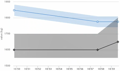
The trend chart displays the following information:
A black curve represents the objectives. If no objective is stored in the trend,
the black curve does not appear.
A gray surface represents the minimum and maximum values of the objective.
A curve in light blue represents the metric value.
A blue surface represents the tolerance value associated to the value.
Click Add to the Timeline.
The information is stored in the analytics magnitude. For more information,
see Add to the Timeline.
To visualize the previous weight analytics, select a trend, Weight
Trend for example, in the list above the trend.
In the list, you can select the following dimensions: Missing
Trend, Threshold Trend, Reaching targets
Trend, Top Human Activity Impact Trend or
Human Activities Solving Trend.
The chart displays a legend
for the metric objectives, the values, and the trend of the selected dimension. For
example, if you select Life Cycle Trend, a legend appears for
the estimated, declared, computed, and measured weight.
The surfaces corresponding to the minimum and maximum values of the objective and to
the tolerance for the metric value, are not displayed.
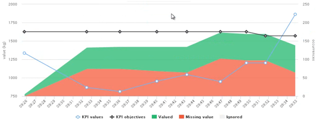
The analytics magnitude is the same as the one of the metric's, including two axes:
time and metric magnitude. When you select Missing Trend, a
third axis called Occurrences appears on the right side of the
timeline chart:
Tip:
Left-click over the chart and drag to zoom in the trend. Click
Reset zoom to switch back to the normal view.
To go back to the weight, center of gravity, and inertia matrix metrics' page, click Global
Scoring.
Display the Prediction Chart
To assess the risks or opportunities for the weight metric,
you can activate a forecast timeline.
Select a metric.
Click Anticipate.
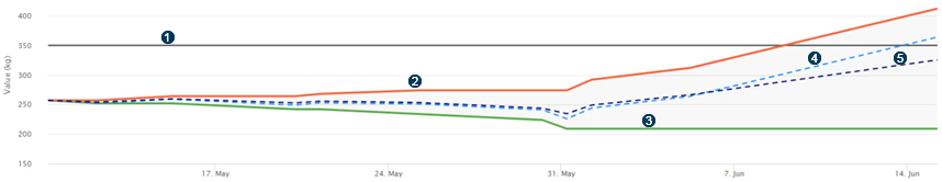
A time chart displays the following information:
Target value line: The black line appears on the chart
when a target exists.
Worst case curve: A combination of all possible
risks.
Best case curve: A combination of all possible
opportunities.
All events occur curve: A combination of opportunities
and risks without considering probabilities.
Statistical Prediction curve: A combination of
opportunities and risks considering their probabilities.
Notes:
You can hover over the points on the red or
green lines to see the risks or opportunities' name and
value.
Compare two Items
You can compare the metrics of two or more selected items. You can also compare
different configurations of an item.
Select two items (or two configurations) in the 3DDashboard and drag them onto Weight and Balance.
There is a tab per items/root.
Click a metric label.
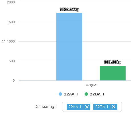
Click Add to Comparison.
Two labels are displayed with the names of the selected items.
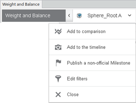
To have access to other commands, click the name of an item.
Click Add to comparison to add the item to the comparison
chart.
A new tab entitled Comparison appears.
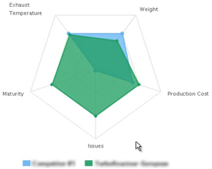
If the number of metrics is equal to two, you obtain a bar chart:
If the number of metrics is more than two, you obtain a spider chart:
Tip:
If you hover over the chart, a tooltip displays the metric values.
To drill down and change the way the chart is displayed, click one of the metrics.
To hide a bar, click its legend at the bottom of the chart.
To remove an item from comparison, click or select
Remove from comparison from the tab's list.
To go back to the weight, center of gravity, and inertia matrix metrics' page, click Global
Scoring.
 and select
Dispatcher, Orpheus Controller and
Orpheus Instance.
You can see blue indicators when the status is valid, or gray indicators when it is not. A tooltip indicates what you should do or provides the index scan date.
and select
Dispatcher, Orpheus Controller and
Orpheus Instance.
You can see blue indicators when the status is valid, or gray indicators when it is not. A tooltip indicates what you should do or provides the index scan date.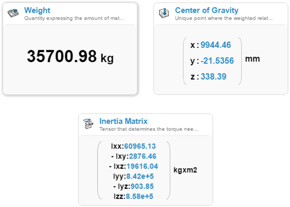
 .
.

 .
.

 from the
  and select
 . It is
indexed in the Cloud View.
. It is
indexed in the Cloud View. 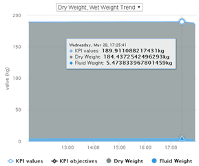
 to
get an assessment of an item from the assembly in a dedicated tab. You can display the
assessment in a pie chart view (default option) or in a multilist view:
to
get an assessment of an item from the assembly in a dedicated tab. You can display the
assessment in a pie chart view (default option) or in a multilist view:
 or
or
 in
the right corner of the panel.
in
the right corner of the panel. .
.


 :
Displays the entire metrics specific to the cockpit in a numbered list. You can
select one or several metrics. Your selection is persistent for the given
widget. At least one metric should be selected, otherwise an error message
appears.
:
Displays the entire metrics specific to the cockpit in a numbered list. You can
select one or several metrics. Your selection is persistent for the given
widget. At least one metric should be selected, otherwise an error message
appears. :
Displays a selection list containing the
:
Displays a selection list containing the  appears to select the ascending or descending order. The sorting is always level by
level.
appears to select the ascending or descending order. The sorting is always level by
level.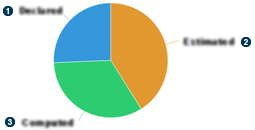
 Declared value of Life Cycle
  Estimated value of Life Cycle
  Computed value of Life Cycle
  .
.
 .
.
 .
.


 .
.
 or select