This example illustrates inelastic deformation of a soil specimen
whose constitutive behavior is modeled with modified Cam-clay plasticity.
The elastic part of the behavior is modeled with both the linear
elastic and porous elastic models. The Cam-clay plasticity theory, which is one
of the critical state plasticity theories developed by Roscoe and his
colleagues at Cambridge, is described in
Plasticity for nonmetals.
Verification of the model is provided by
Triaxial tests on a saturated clay.
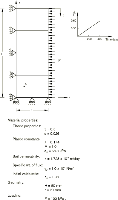
The geometric configuration is one of the most common soils tests: a
triaxial specimen, confined by an enclosing membrane, being squeezed axially
between platens (see
Figure 1).
Perfectly smooth and perfectly rough platens are both considered. The platen
motion is assumed to be very slow compared to characteristic diffusion times in
the soil, and the platen is assumed to provide perfect drainage, so that the
pore pressures throughout the soil specimen are always essentially zero. Pore
fluid diffusion is, thus, not a significant effect in this case. See
The Terzaghi consolidation problem
and
Plane strain consolidation
for cases where transient effects in the pore fluid diffusion are an important
aspect of the overall response.
As the specimen is compressed, the elastic-plastic response of the specimen
consists of two competing effects. Elastically, the increased compressive
hydrostatic effective stress on the soil skeleton causes a stiffening of the
response. When the soil yields, inelastic deformation results in softer
behavior. Eventually the stress state in some region of the specimen reaches
critical state, where the soil skeleton response is perfectly plastic. When
this region is sufficiently developed, a limit state is attained, and the
specimen's resistance to further compression no longer increases. The analysis
is intended to track the response from the initial loading to this limit state.
Problem description
The soil sample is an axisymmetric cylinder, as shown in
Figure 1.
The model takes advantage of symmetry about the midplane, as well as the
axisymmetry of the configuration. The specimen has a length to diameter ratio
of 3. Two cases are considered: one in which the platen is assumed to be
perfectly smooth, so that the stress state in the specimen will be homogeneous,
and one in which the platen is assumed to be completely rough, so the soil in
contact with the platen cannot move with respect to the platen. This latter
case results in an nonhomogeneous stress state, as the specimen bulges during
compression. The eight element mesh shown in
Figure 1
is not expected to capture this nonhomogeneous state accurately but should
suffice for the present demonstration purposes.
The material properties of the soil are based on the example used by
Zienkiewicz and Naylor (1972). The properties for the Cam-clay model with
porous elasticity are shown in
Figure 1.
The Cam-clay model with linear elasticity uses a Young's modulus of 15 GPa.
This value is based on the elastic stiffness (at the end of the loading step)
of the examples that use porous elasticity.
Initial conditions
The Cam-clay model assumes that the soil has no stiffness at zero stress, so
that some initial (compressive) stress state must be defined for the material.
In this case we assume that the soil sample is under an initial hydrostatic
pressure of 0.1 MPa (14.5 lb/in2), and this confining pressure
remains constant throughout the test. Since the soil may drain through the
platen, this pressure is carried as an effective stress in the soil skeleton.
This initial stress state is defined using initial conditions. In this
particular example it is trivial to see that this initial stress state is in
equilibrium with the external distributed pressure of the same magnitude. In
more complex cases it may not be so simple to ensure that the discrete, finite
element model is in equilibrium with the geostatic loading. Accordingly, the
first step of any analysis involving an initial stress state should be a
geostatic step. In that step the geostatic external loads (in this case the
pressure on the specimen) should be specified.
Abaqus
will then check whether the initial stress state is in equilibrium with these
loads. If it is not,
Abaqus
will iterate and attempt to establish an equilibrium stress field that balances
the prescribed tractions. Such iteration does not occur in this case since the
prescribed initial stress is in equilibrium with the applied tractions.
Loading
The specimen is compressed to 40% of its initial height over 34.56 ×
106 sec (400 days). Although this represents a large strain of the
specimen, geometric nonlinearity is ignored in this example because we wish to
examine the effects of the material nonlinearity, and we only report the
stress-strain response at points, rather than overall load-deflection response
that will be predicted quite inaccurately unless geometric nonlinearity is
included. The loading is applied in a transient soils consolidation step
specifying the time period, with an associated boundary condition prescribing
the travel of the platen during that time. The platen is assumed to drain
freely throughout the analysis. This is specified by a boundary condition,
fixing the pore pressure at zero on the top edge of the mesh. The loading is
intended to represent very slow compression, sufficiently slow that the pore
pressures never rise to any significant values. We can obtain a rough idea of
this time scale by noting that a characteristic time for pore pressure
dissipation is ,
where H is a typical dimension from the draining surface
(60 mm, 2.362 in, in this case);
is the specific weight of the pore fluid (1.0 × 10⁴ N/m3,
0.0369 lb/in3); k is the permeability of the
soil (0.1728 mm/day, 6.803 × 10⁻³ in/day); and
is a typical soil modulus, which we compute as ,
where
is the logarithmic bulk modulus and p is a typical mean
normal effective stress. T is, thus, estimated as 0.05
days. This is about the time it takes for pore pressures to drop to 5% of their
initial values, following sudden application of a load (see Terzaghi and Peck,
1967). Since the time scale chosen for the loading of the test specimen in this
example is very long compared to this value, no significant pore pressures
should ever arise in the analysis.
The same analysis could be performed by using a static procedure, in which
case the coupled, effective stress formulation element type could be replaced
with an element that models soil deformation only. We choose to use the coupled
element type and the soils consolidation procedure to exercise these features.
The accuracy of the equilibrium solution within a time increment is
controlled by iterating until the out-of-balance forces reduce to a small
fraction of an average force magnitude calculated internally by
Abaqus.
The rough platen causes an nonhomogeneous stress state, which tends to cause an
underestimation of this average force magnitude since stresses are locally
higher in the region of the mesh near the platen and the reference force
magnitude is averaged over the entire mesh. To avoid iterating to excessive
accuracy, we have overridden the default calculation of the average force
magnitude and have defined that typical actual nodal forces will be of the
order 100 N (22.52 lb). This is done using solution controls. The increment
size choice is automatic, determined by allowing a maximum pore pressure change
()
of 0.16 KPa (.023 lb/in2) per increment, which should give
sufficient definition of the solution.
Results and discussion
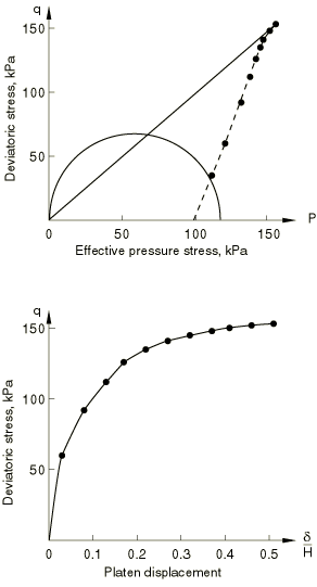
Figure 2
shows results for the rough platen case, when the stress field is
nonhomogeneous, and shows results corresponding to point A
in
Figure 1:
this is the stress output point at the centroid of the element shown.
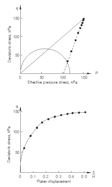
Figure 3
is for the smooth platen case, when the stress field is homogeneous. The top
section of each figure shows the –q
plane. Here p is the equivalent effective pressure stress,
defined by
and q is the equivalent deviatoric stress (the Mises
equivalent stress) defined by
where
is the deviatoric stress (here
is a unit matrix).
The
plot in each case shows the critical state line, the initial yield surface, and
the stress trajectory followed in the solution. The bottom section of each
figure is a plot of the equivalent deviatoric stress, q,
versus the vertical deflection of the platen. The behavior in both cases is as
we would expect: a gradual softening of the specimen after yield, until
critical state is reached, when the behavior becomes perfectly plastic. In the
rough platen case, the response at the point plotted moves some way up the
critical state line after it reaches that line: presumably this is because
other points in the model have not yet reached the limit state.
Similar results are obtained for the Cam-clay model with linear elasticity.
Rough platen case using the linear elasticity model with CAX8RP elements. This analysis is done as basic verification of the
Cam-clay model with linear elasticity.
The only change needed for the smooth platen case is to remove the boundary
conditions in the radial direction at the top of the mesh.
References
Terzaghi, K., and R. B. Peck, Soil
Mechanics in Engineering
Practice, John Wiley and
Sons, New
York, 2nd, 1967.
Zienkiewicz, O.C., and D. J. Naylor, “The
Adaptation of Critical State Soil Mechanics Theory for Use in Finite
Elements,” Stress-Strain Behavior of
Soils, edited by R. H. G. Parry, G. T. Foulis and
Co., Ltd., London,
1972.
Figures
Figure 1. Triaxial consolidation: geometry, properties, and loading. Figure 2. Shear stress versus mean normal stress and axial strain. Rough platen
case. Figure 3. Shear stress versus mean normal stress and axial strain. Smooth platen
case.