The bumper analysis is a two-step process. In the first step the
interference between the bumper's inner diameter and the mandrel is resolved.
In the
Abaqus/Standard
analysis the automatic “shrink” fit method (see
Common Difficulties Associated with Contact Modeling in Abaqus/Standard)
is used: the calculated initial penetration is allowed at the beginning of the
step and scaled linearly to zero at the end of the step. In the
Abaqus/Explicit
analysis the interference resolution step is performed in one of three ways. In
the first approach the initial penetration is solved using the "shrink” fit
method (the same as in the
Abaqus/Standard
analysis). In the second approach the mandrel is positioned so that no contact
or overclosure exists between the bumper and the mandrel at the outset of the
analysis. The rigid surface representing the mandrel is then moved in the
radial direction to simulate the compression of the bumper due to the
interference fit. In the third approach the shrink fit solution from
Abaqus/Standard
is imported into
Abaqus/Explicit.
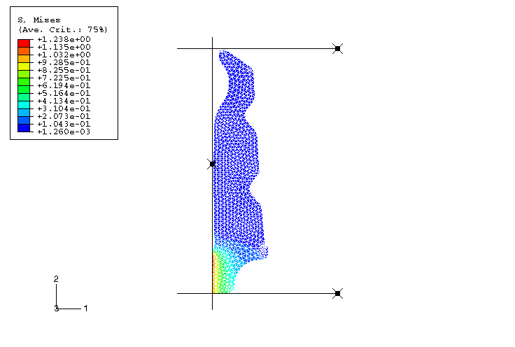
A comparison of the Mises stresses predicted by
Abaqus/Standard
and
Abaqus/Explicit
at the end of the interference step shows that the results are very similar
(see
Figure 3
and
Figure 4).
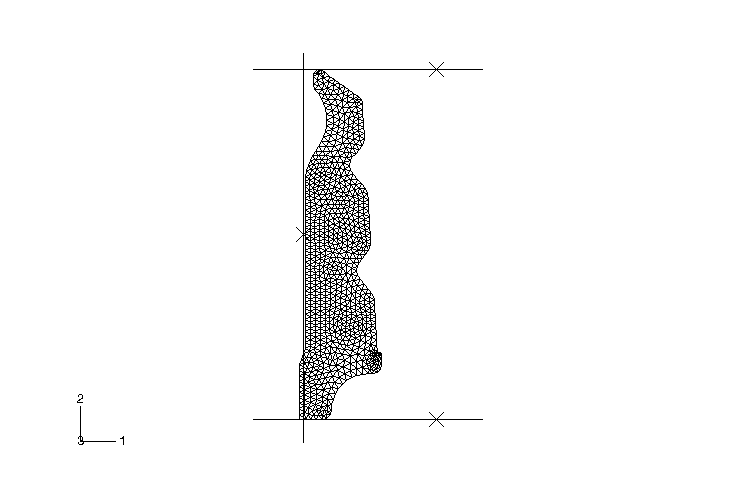
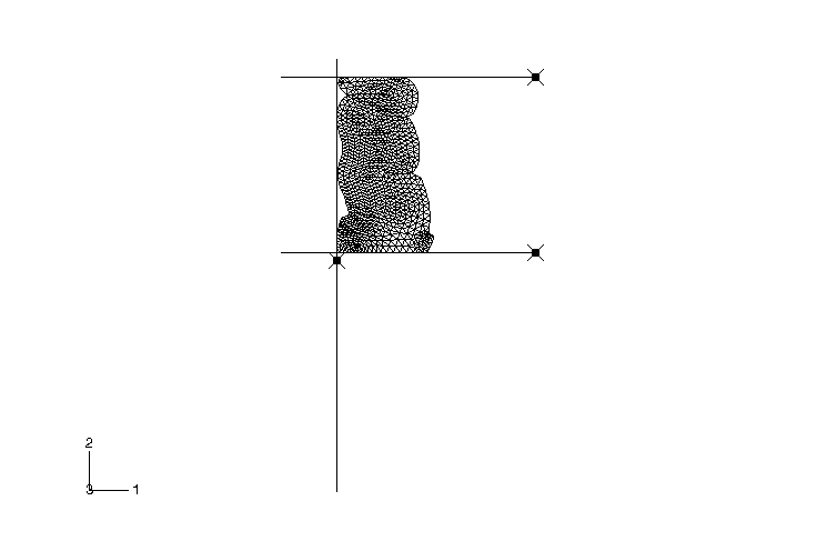
In the second step the bottom surface compresses the bumper 42.0 mm (1.7 in)
as a result of the application of displacement boundary conditions to the
reference node of the surface.
Figure 5,
Figure 6,
and
Figure 7
show the final deformed shape of the bumper; the high compressibility of the
material is apparent, as well as the folding of the surface onto itself.
Although a general knowledge of where the folding would occur was used in the
definition of the self-contacting surfaces, it is not necessary to know exactly
where the kinks in the surface will form.
The final deformed shapes predicted by
Abaqus/Standard
and
Abaqus/Explicit
for the CAX3 element mesh are the same (see
Figure 5
and
Figure 6,
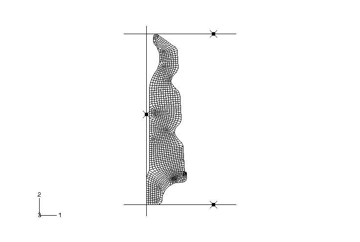
respectively). A similar shape is predicted by
Abaqus/Explicit
when CAX4R elements are used (see
Figure 7).
However, the solution obtained with CAX4R elements in
Abaqus/Explicit
reveals that local buckling occurs in the upper-left folding radius. This makes
a similar analysis using CAX4R elements in
Abaqus/Standard
very difficult. The local buckling is not captured in the CAX3 analysis due to the stiffer nature of these elements.
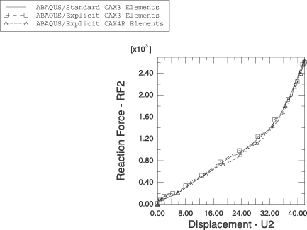
The load versus displacement curves of the bottom surface are shown in
Figure 8.
The results obtained with CAX3 elements in
Abaqus/Standard
and with CAX3 and CAX4R elements in
Abaqus/Explicit
are very similar. The energy absorption capacity of the bumper is seen through
these curves.