Coupled thermomechanical analysis of viscoelastic dampers
This example examines the response of a viscoelastic damper under cyclic loading with the damper material modeled as a linear viscoelastic material using a Prony series calibrated to capture the hysteresis response accurately.
The following Abaqus features and techniques are demonstrated:
using Prony-series viscoelasticity to account for material hysteresis,
using the thermorheologically simple (TRS) material model to account for temperature dependence in a viscoelastic material,
accounting for heat generated by mechanical energy dissipation through coupled temperature-displacement analysis, and
comparing the response of a structure experiencing large deformations using elastic or hyperelastic material models.
One tool commonly used in Abaqus to model stress relaxation in viscoelastic materials is the Prony series. However, using the Prony series to model stress relaxation in dissipating materials often leads to underprediction of the size of the hysteresis loop for the material when subjected to cyclic loading (Dalrymple et al., 2007). If both the stress relaxation and hysteretic behavior of a given material must be modeled accurately, a more complicated material model, such as the parallel rheological framework model, is required. However, in some structures the stress relaxation response may be of secondary importance to the hysteretic energy dissipation under cyclic loading. In such cases it can be reasonable to calibrate the Prony series coefficients in a manner that accurately captures the hysteresis response of the material at the expense of accurately modeling the stress relaxation response. In this example the response of a viscoelastic damper under cyclic loading is examined. The damper material is modeled as a linear viscoelastic material with a Prony series calibrated to capture the hysteresis response accurately.
One of the salient characteristics of damping materials is their ability to convert mechanical energy into other forms of energy, typically heat. However, the mechanical response of these materials is often highly sensitive to temperature. This analysis examines the importance of accounting for the interdependence of heat generation and transport with mechanical response through the use of a fully coupled thermomechanical analysis.
Geometry
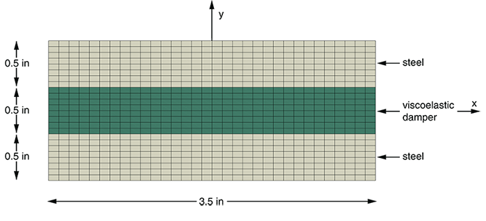
The model consists of a layer of viscoelastic damping material between two steel plates, as shown in Figure 1. The damper dimension is 3.5 inches in the x-direction, and the viscoelastic material and steel plates are each 0.5 inches thick, for a total dimension of 1.5 inches in the y-direction.
Materials
The model contains two materials, steel and a viscoelastic damping material with a response described by Shen and Soong (1995). Details of the material response are provided in Materials below.
Initial conditions
The initial temperature in the structure is uniformly 21.7 °C.
Boundary conditions and loading
The damper is subjected to sinusoidal shear loading at a rate of 1 Hz for a period of 10 seconds such that the nominal engineering shear strain in the viscoelastic damping material has an amplitude of approximately 50%. This loading is imposed by specifying the displacement of the top surface.
For heat conduction, the damper’s boundaries are assumed to be adiabatic (i.e., no heat is transferred to or from the environment).
Abaqus modeling approaches and simulation techniques
Four analyses are performed comparing the predicted response if heat generation from mechanical dissipation is or is not accounted for and comparing the effect of modeling the viscoelastic damping material as a linear elastic or hyperelastic material.
Summary of analysis cases
Case 1
Quasi-static stress analysis with linear elasticity for the viscoelastic damper material
Case 2
Quasi-static stress analysis with hyperelasticity for the viscoelastic damper material
Case 3
Coupled temperature-displacement analysis with linear elasticity for the viscoelastic damper material
Case 4
Coupled temperature-displacement analysis with hyperelasticity for the viscoelastic damper material
Analysis types
Two types of analyses are performed: a transient, static, stress/displacement analysis that neglects the generated heat and a coupled transient temperature-displacement analysis. Both analysis types neglect inertial effects (i.e., the model is quasi-static) and use general steps with geometric nonlinearity since the model undergoes large displacements. In the coupled analysis (see Fully Coupled Thermal-Stress Analysis), transient heat transfer resulting from heat generated by dissipation of mechanical energy is modeled along with the force-displacement. The resulting temperature changes will affect the structure’s response due to material temperature dependence in the viscoelastic damper and thermal expansion.
Mesh design
A single mesh refinement is examined, with 8 elements through the thickness of each layer of the damper (resulting in a total of 24 elements in the y-direction) and 32 elements in the x-direction. Plane strain is assumed. CPE4 and CPE4H elements are used for the stress analysis for the steel and viscoelastic damper materials, respectively. The coupled analysis uses CPE4T and CPE4HT elements.
Materials
This section provides the properties used for the various materials in the model.
Steel
The steel’s mechanical response is modeled with linear elasticity. The Young’s modulus of the steel is psi, and the Poisson's ratio is .
Viscoelastic damper
The mechanical response of the viscoelastic damper material is determined from experimental data provided by Shen and Soong. For temperature dependence, the material is assumed to be thermorheologically simple. Shen and Soong provide the following TRS shift function based on temperature:
which is a simplified form of the Williams-Landell-Ferry (WLF) relationship implemented within Abaqus (see Time Domain Viscoelasticity):
The form of the TRS shift function given by Shen and Soong can be replicated using the WLF relationship by selecting values of and such that and . Therefore, the parameters of the WLFTRS definition of the material implemented within Abaqus are defined as °C, , and °C.
The storage and loss moduli along with the corresponding frequencies from Shen and Soong were shifted using the TRS shift function to a reference temperature of 21.7 °C. This choice of reference temperature, which in practice is arbitrary, was made based on the temperature at which the regression performed by Shen and Soong yields no shift. The original moduli, along with the shifted values, are given in Table 1. As a general practice, it is important that the time scales or frequencies of the loading in the analysis be within the scope of the time scales and frequencies of the experimental data used to characterize the material response. The loading in this analysis is 1 Hz, which is within the range of frequencies given in Table 1.
The Levenburg-Marquardt algorithm (Press et al., 1992), a least-squares approach, was used to obtain the Prony series parameters (see Table 2) for the Maxwell model using the temperature-shifted frequencies and storage and loss moduli. The initial shear modulus is 2.0845 ksi.
For the instantaneous elastic response of the material, it is assumed that the bulk modulus is constant with respect to time or frequency. The material is assumed to be nearly incompressible with an initial Poisson’s ratio of 0.495. This results in a bulk modulus of ksi.
This example compares two different approaches for modeling the instantaneous elastic response of the damping material. The first is to model the response as linear. The initial Young’s modulus of E = 6.232 ksi is determined from the initial shear modulus and Poisson’s ratio.
The second approach utilizes a neo-Hookean hyperelastic material definition (see Hyperelastic Behavior of Rubberlike Materials). Hyperelasticity is based on finite deformation theory, which may be more appropriate for this model considering the large strains that are experienced. Another consequence of this change is that the stress-strain relationship for the material will be nonlinear. The neo-Hookean model is chosen due to the lack of comprehensive data for the instantaneous stress-strain response of the viscoelastic damping material. The strain energy potential constants ( and ) are determined from the initial shear and bulk moduli.
Heat transfer
The properties of the materials related to heat transfer are given in Table 3. The inelastic heat fraction (see Fully Coupled Thermal-Stress Analysis) for the viscoelastic damper material is specified as . This assumes that all energy dissipated by viscoelasticity is converted into heat and accounts for the change of energy units from in-lbf in the mechanical analysis to BTUs, which are used to define the material properties related to heat transfer given in Table 3.
Initial conditions
The initial temperature of all nodes is 21.7 °C.
Boundary conditions
The nodes on the top surface are constrained in the y-direction. The nodes on the bottom surface are constrained in both the x- and y-directions. No thermal boundary conditions are specified, meaning that there is no heat transfer with the environment.
Loads
A sinusoidal time-varying x-direction displacement with an amplitude of 0.25 inches and a frequency of 1 Hz is applied to the nodes on the top surface.
Convergence
Adaptive time stepping is used with a creep strain error tolerance (CETOL) of 5 × 10⁻³. Increments that are sufficiently small to satisfy this tolerance typically converge within 2–3 iterations.
Discussion of results and comparison of cases
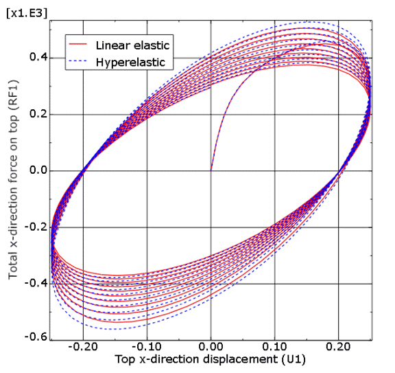
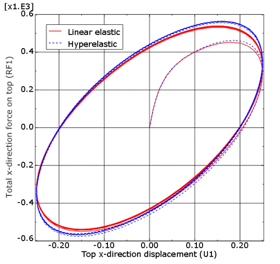
Figure 2 shows a contour of the logarithmic shear strain in the damper at the maximum stroke of the final cycle in the coupled model using hyperelasticity, showing the large deformations present in the viscoelastic damper material. The hysteresis responses predicted using the two different material models are shown in Figure 3 for the coupled thermomechanical analysis and Figure 4 for the uncoupled stress analysis. The importance of accounting for the heat generated by dissipation of mechanical energy is immediately apparent in the way that the hysteresis loops flatten and decrease in area over time in the coupled analyses. These changes occur because the material loses stiffness as the temperature increases. No such decrease is noted in the pure stress analysis—the cyclic hysteresis response reaches a steady state after a single cycle has been completed.
Figure 3 and Figure 4 show that the forces are slightly higher when using the hyperelastic model for the damping material than when using the linear elastic model. This difference is expected due to the nonlinear nature of the stress-strain relationship obtained using hyperelasticity and the use of finite deformation theory.
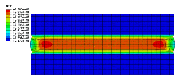
Figure 5 shows the contour of the temperature in the damper, indicating that some regions of the damper experience a temperature increase of approximately 8 degrees over the 10-second duration of the analysis. This increase is due to the heat generated by mechanical energy dissipation. The generated heat accumulates in the viscoelastic material faster than it is conducted to the cooler steel plates, leading to a steady temperature increase. Figure 6 shows the time history of the temperature at the central node (node 1217) of the damper in the coupled analysis. The temperature rise is more pronounced in the model using hyperelasticity due to the higher stresses (and subsequently greater energy dissipation) experienced when using the hyperelastic material definition.
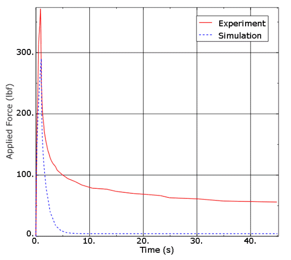
One additional aspect of interest for this material definition is how the predicted stress relaxation compares to the material’s actual response. Recall that for this viscous damper, the hysteresis response is of primary interest. Therefore, the viscoelastic Prony series was calibrated to capture that aspect of the material response accurately. Shen and Soong performed relaxation experiments on a test fixture using the material in this example. The force response of that test fixture can be approximated using the model from this example by multiplying the sum of the x-direction reaction forces in the upper nodes of the model by 5, permitting a direct comparison between experiment and simulation.
Figure 7 compares the time history of the experimentally measured and simulated reaction forces resulting from loading the damping material to a nominal engineering shear strain of 20% over one second and then holding the displacements of the test fixture constant. As seen in the figure, the force in the simulation drops more quickly than it does in the experiment, and to a much lower value. This result highlights the intrinsic limitation of linear viscoelasticity described in the introduction of this example—it is generally not possible to represent both the hysteresis response and the stress relaxation response accurately using a linear viscoelastic Prony series. Therefore, while the approaches described in this example are appropriate for modeling a viscoelastic material under cyclic loading, the approach described here is not recommended for analyses in which stress relaxation is of primary importance.
Acknowledgements
SIMULIA would like to thank Professor Gary Dargush at SUNY Buffalo for providing the model used in this example, which is based on work by Rajesh Radhakrishnan (2000).
Dalrymple, T., J. Choi, and K. Miller, “Elastomer Rate-Dependence: A Testing and Material Modeling Methodology,” 172nd Technical Meeting of the Rubber Division of the American Chemical Society, Cleveland, OH, pp. 1–16, 2007.
Press, W. H., S. A. Teukolsky, W. T. Vetterling, and B. P. Flannery, Numerical Recipes in Fortran, 172nd Technical Cambridge University Press, Cambridge, U.K, 1992.
Radhakrishnan, R., Coupled Thermomechanical Analysis of Viscoelastic Dampers, Master's Thesis, State University New York, Buffalo, NY, 2000.
Shen, K. L., and T. T. Soong, “Modeling of Viscoelastic Dampers for Structural Applications,” Journal of Engineering Mechanics, vol. 121, issue 6, pp. 694–701, 1995.
Tables
Table 1. Original and shifted storage and loss moduli from Shen and Soong (1995).
(°C)
f (Hz)
G (ksi)
G (ksi)
fr (Hz)
Gr (ksi)
Gr (ksi)
21
1
0.199
0.259
1.096
0.199
0.258
1.5
0.265
0.326
1.644
0.264
0.325
2
0.3
0.395
2.192
0.299
0.394
2.5
0.365
0.463
2.74
0.364
0.462
3
0.386
0.487
3.288
0.385
0.486
32
1
0.093
0.128
0.265
0.09
0.124
1.5
0.1
0.158
0.398
0.097
0.153
2
0.131
0.189
0.53
0.127
0.183
2.5
0.147
0.213
0.663
0.142
0.206
3
0.182
0.242
0.795
0.176
0.234
38
1
0.074
0.09
0.122
0.07
0.085
1.5
0.068
0.102
0.183
0.064
0.097
2
0.1
0.114
0.244
0.095
0.108
2.5
0.106
0.125
0.305
0.1
0.119
3
0.114
0.14
0.366
0.108
0.133
Table 2. Prony series parameters.
s
s
s
Table 3. Thermal properties.
Quantity
Steel
Viscoelastic Damper
Density (lbf-s2/in4)
Thermal expansion (in/in-°C)
Thermal conductivity (BTU/s-in-°C)
Specific heat (BTU-in/lbf-s2-°C)
76.3
300
Figures
Figure 1. Viscoelastic damper geometry. Figure 2. Shear component of the log strain at t=9.25 s for the coupled temperature-displacement model using hyperelastic materials. Figure 3. Hysteresis response for the coupled thermomechanical analysis. Figure 4. Hysteresis response for the pure stress analysis (no thermal coupling). Figure 5. Temperature contour in fully coupled model with hyperelasticity at t=10 s. Figure 6. Temperature history at center of viscoelastic region for coupled analysis. Figure 7. Comparison of relaxation response from experiments by Shen and Soong with prediction using material calibrated to capture hysteresis response.