The Radial Base Function Model

RBF networks are characterized by reasonably fast training and reasonably compact networks.

Weissinger (1947) was the first to use numeric potential flow to calculate the flow around wings. The potential flow equations are a radial basis function. Hardy (1971) realized that the same concept could be used to fit geophysical data to geophysical phenomena. Broomhead and Lowe (1988) renamed this technology “neural nets,” and it was subsequently used to approximate all types of behavior.

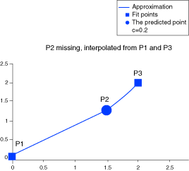
Results Analytics follows the Hardy (1972, 1990) method as described by Kansa (1999).

Let $x_1,\dots ,x_N\in \mathrm{\Omega }\subset {\mathfrak{R}}^N$ be a given set of nodes. Let $g_i(x)\equiv g(\Vert x-x_j\Vert )\in \mathfrak{R},j=1,\dots ,N$, be a set of any radial basis functions. Here $\Vert x-x_j\Vert$ is the Euclidian distance given by ${(x-x_j)}^T(x-x_j)$. Given interpolation values $y_1,\dots ,y_N\in \mathfrak{R}$ at data locations $x_1,\dots ,x_N\in \mathrm{\Omega }\subset {\mathfrak{R}}^N$, RBF interpolant

is obtained by solving the system of $N+1$ linear equations

for $N+1$ unknown expansion coefficients ${\alpha }_j$.

Hardy, the primary innovator of the RBF Method, adds a constant to the expansion and constraints the sum of the expansion coefficients to zero as seen in Eqn 1 and Eqn 2, introducing the notation

$\alpha ={({\alpha }_1,\dots ,{\alpha }_{N+1})}^{\mathrm{T}}$, and $y={(y_1,\dots ,y_N,0)}^T\in {\Re }^{N+1}$ $\in {\mathfrak{R}}^{N+1}$. We can rewrite the system (Eqn 2) in the matrix form as

Then the interpolation expansion coefficients are given by

You can easily find the derivatives of the interpolant at the nodes $x_1$. For example,

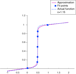
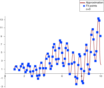
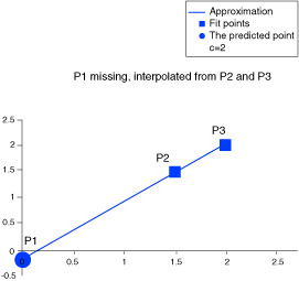
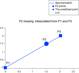
Because the physics of the model can vary, a different type of basis function would be needed to provide a good fit. The response surface goes through all the given interpolation data.

Results Analytics uses a variable power spline basis function that can be tuned to approximate a large number of other functions.

A variable power spline radial basis function is given by

where $\Vert x-x_j\Vert$ is the Euclidian distance and $c$ is a shape function variable between 0.2 and 3 (i.e., $\mathrm{0.2.}<c<3$).

For a value $c=\mathrm{1.15}$, a good approximation of a step function can be achieved with just seven interpolation points. For a value of $c=2$, a good approximation of a linear function can be achieved with just three interpolation points, as shown in the following figure:

For a value $c=3$, a good approximation of a harmonic function is achieved with about seven points per harmonic period.

Picking $c=3$ for the step function example would produce an approximation that would go through the seven data points, but it would more resemble a single sine wave than a step function. There are obviously an infinite number of solutions that will go through any given set of data points.

In most of the literature this problem is solved by splitting the interpolation data into two groups. One group is used to create the radial basis function approximation, and one group is used to compute the error between the radial basis function approximation for those points and the actual function values. The shape function is optimized to minimize the summed errors. This is a valid approach when a lot of data points are available for the interpolation; however, typical design problems in Results Analytics deal mostly with very sparse data sets, and it seems inefficient to use only half the data to create the actual response surface.

Results Analytics uses a different approach by defining a good fit when the shape of the curve does not change when a point is subtracted. Results Analytics optimizes the value of $c$ for a minimum sum of the errors for $N-1$ data points.

This approach can be illustrated by reviewing the graph of the straight line approximation below (P1 missing) the point P1 is approximated using the points P2 and P3; in the graph below (P2 missing) the point P2 is approximated from the two extreme points P1 and P3. For $c=2$, the sum of the errors for the “missing points” is low as seen in the figure.

For $c=0.2$, the sum of the errors of the “missing points” is extremely high.

You can use the smoothing filter to relax the requirement that the Radial Base Function Model (RBF) approximation passes through every single data point.

The primary purpose of the smoothing filter is to smooth out noisy data. By not going through every point, Results Analytics can effectively smooth noisy functions and provide an approximation that may be easier to optimize. The value specified by this option averages the output values of points that are clustered in the normalized filter domain.

The filter operates in the Euclidian space with domains normalized to [0,1]. Clustering is performed within that domain. For example, consider an approximation with a single input $x$, where $0<x<10$. For a smoothing filter value of 0.001, Results Analytics clusters and averages all points in the range of $0.719<x<0.721$ for the input at $x=7.2$ (the space $x$ is normalized over the range 10).

Results Analytics sets the default value of the smoothing filter to 0.0. You can change the value when you create an approximation using the Radial Base Function Model.

The maximum allowed value for the smoothing filter is 0.1. Mathematically, this means you have a maximum of 10 clustered sample points for each input. (Through research, it has been determined that at larger values it does not make sense to perform an RBF.) With 10 clustered sample points, Results Analytics can identify a maximum of four local minima (sine wave) across one dimension. With quartic RSM Results Analytics can identify three local minima across one dimension. Therefore, if you have to use a smoothing filter value greater than 0.1, it is better to use the RSM technique.

There is no theoretical basis to distinguish between signal and noise in the data used for approximation. It is recommended that you evaluate the resultant RBF to determine if this option is appropriate for your application.